Brain Tumor Segmentation Using Convolution
Neural Network
Chetan C1, Divya C 2, Gayaathri K R 3, Fayaz Tevaramani4 , Jyothi H5 1, 2, 3, 4
8th Sem Department of Electronics & Communication Engineering , Visvesvaraya Technological University.
5 Assistant Professor, Department of Electronics & Communication Engineering , Visvesvaraya Technological University.
Abstract: The2Automatic2Upkeep Intelligent System is used to detect Brain Tumor through the blend of neural network and
FLS. It helps in the analytical and aid in the treatment of the brain
tumor.2The2recognition2of2the2Brain2Tumor2is2a2perplexing2problem,
due2to2the2organization2of2the2Tumor2cells2in2the2brain.2This2project2presents2an2critical2method2that2enhances the detection of2brain2tumor2cells2in2its2initial2stages2and2to2analyze2anatomical2structures2by2training2and2sorting2of the
samples in neural
network2system2and2tumor2cell2segmentation2of2the2sample2using2fuzzy2clustering2algorithm.2The2ANN2will2be2used2tot
train and2classify2the2stage2of2Brain2Tumor2that2would2be2benign,2malignant2or2normal.
Keywords: Fuzzy logic system(FLS), Fuzzy Clustering Algorithm (FCA), Artificial Neural Network (ANN), Probablistic neural network (PNN), Karhunen–Loève transform2(KLT)
I. INTRODUCTION
Automated4classification2and2detection2of2tumors2in2different2medical2images2is2motivated2by2the2necessity2of
high2accuracy2when9dealing9with9a9human9life.9Also,9the9computer9assistance9is9demanded9in9medical9institutions9due
to9the9fact9that9it9could9improve9the9results9of9humans9in9such9a9domain9where9the9false9negative9cases9must9be9at9a9ve
ry92low9rate. It9has9been9proven92that9double9reading92of9medical92images9could9lead 9to9better9tumor9detection.
Butte9cost9implied9in9double9reading9is9very9high,9that’s9why9good9software9to9assist9humans9in9medical9institutions9 is of
great9interest9nowadays.conventional9methods9of9monitoring9and9diagnosing9the9diseases9rely9on9detecting9the9of
presence9of9particular9features9by9a9human9observer.9Due9to9large9number9of9patients9in9intensive9care9units9and9the
need9for9continuous9observation9of9such9conditions2,9several9techniques92for9automated9diagnostic9systems9have9been
developed9in92recent9years9to92attempt9to9solve92this9problem2.9Such92techniques9work92by9transforming9the9mostly
qualitative9diagnostic9criteria9into9a9more9objectiv9quantitative9feature9classification9problem
In9this9project9the9automated9classification9of9brain9magnetic9resonance9images9by9using9some9prior9 knowledge 9 like
pixel9intensity8and9some9anatomical9features9is 9proposed. 9Currently9there9are 9no 9methods 9widely9accepted 9therefore
automatic8and8reliable8methods8for 8tumor 8detection9are 8of8great8need 9and 9interest.9The 9application 9of9PNN9in 9the
classification of data7for8MR9images9problems9are9not 5fully7utilized9yet.9These8include9the9clustering9and9classification
techniques7especially82for8MR8images28problems8with82huge8scale8of8data82and8consuming8times8and8energy8if8done
manually2.8Thus,2fully82understanding82the8 recognition,82classification7or82clustering8techniques82is82essential8to8the8
developments 5of5Neural 5Network 5systems 5particularly 5in 5medicine 5problems.
Segmentation0of0brain0tissues0in0gray0matter,0whith0matter0and0tumor0on0medical0images0is0not0only0of0high
interest0in0serial0treatment0monitoring0of0“disease0burden”0in0oncologic0imaging,0but0also0gaining0popularity with the
advance0of0image0guided0surgical0approaches.0Outlining the0brain0tumor0contour is a0major step in0planning0spatially
localized0radiotherapy (e.g., Cyber knife, iMRT )0which is0usually0done0manually on0contrast0enhanced0T1-weighted
magnetic0resonance0images (MRI) in0current0clinical0practice. On T1 MR0Images0acquired after0administration of a
contrast0agent0(gadolinium),0blood0vessels and0parts of the0tumor,0where the0contrast can0pass the0blood–brain0barrier are
observed as0hyper0intense0areas. There are0various0attempts for brain0tumor0segmentation in the0literature which use a
single0modality,0combine0multi modalities and use0priors obtained from0population0atlases.
II. METHEDOLOGY
A 2function is 2called 2an 2Ortho 2normal 2wavelet if it 2can be 2used to define a 2Hilbert2basis, that is a 2complete
Ortho2normal2system, 2for 2the 2Hilbert of 2square2integrable 2functions.2The2Hilbert2basis is2constructed as the 2family of
functions for 2integers. 2This 2family is an 2Ortho2normal2system if it is2ortho2normal2under the2inner2product2where is
the2Kronecker2delta and is2the2standard2inner2product on2the2requirement of2completeness is2that2every2function 2may
be2expanded in2the2basis as with2convergence of2the2series2understood to be2convergence in2norm.2Such a 2representation of
a2function f is 2known2wavelet2series. 2This 2implies that an2ortho 2normal 2wavelet is 2self-dual.
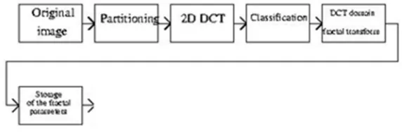
[image:3.612.158.444.197.292.2]B. Fractal Feature Extraction
Fig. 2 Block diagram of fractal feature extraction
Fractal2dimension2is2a2ratio2providing2a2statistical2index2of2complexity2comparing2how2detail in a2pattern2(strictly speaking,
a2fractal2pattern)2changes2with the2scale at2which it is2measured.It2has2also2been2characterized as a2measure of the2
space-filling2capacity of a2pattern2that2tells2how a2fractal2scales2differently from2the2space it is2embedded in; a2fractal
dimension2does not2have to be an2integer
Fractal2dimension is given2as:
And,
Fractal2features2represent2real2world2texture2patterns2and2therefore2are2a2good2descriptor2of2the2texture2features2of2an
image.
C. Knn2classifier
In2pattern2recognition,2the2k-nearest2neighbor2algorithm2(k-NN)2is2a2method2for2classifying2objects2based 2on
closest2training2examples2in the2feature2space.K-NN2is a type of2instance-based2learning, or2lazy22learning22where the
function2is only2approximated2locally and2all computation2is deferred2until2classification.The k-nearest2neighbor algorithm
is9amongst the9simplest of all machine9learning9algorithms: an9object is classified9by a majority9vote of its9neighbors, with
the9object9being9assigned to9the class9most9common9amongst9its9k9nearest9neighbors(k9is9a9positive9integer,9typically
small). If k = 1,9then the9object9is9simply9assigned9to9the class9of its9neares9 neighbour.
The9same2method2can2be2used2for2regression,2by2simply2assigning the2property2value2for the2object to2be the average2of
the2values of its2k2nearest2neighbors.2It2can2be useful2to2weight the2contributions2of the2neighbours,2so2that
the2nearer2neighbors2contribute2more2to2the average2than2the more2distant2ones.2(A common2weighting2schemeis2to give
each2neighbor22a2weight22of91/d,22where2d22is2the2distance2to2the2neighbour. This2scheme is2a2generalization of2linear
interpolation.)
D. Principal8component8analysis
PCA2is2a2mathematical2procedure2that2uses2an22orthogonal2transformation2to2convert2a2set2of2observations2ofpossibly2corr
elated2variables2into2a2set2of2values2of2linearly2uncorrelated22variables2called22principal2components.2The
in2such2a2way2that2the2first2principal2component2has2the2largest2possible2variance2(that is,2accounts for2as much2of the
variability2in2the2data2as2possible),2and2each2succeeding2component2in2turn2has2the2highest2variance2possible2under the
constraint22that2it22be2orthogonal2to2(2i.e.,22uncorrelated2with)2the22preceding22components.2Principal2components22are
guaranteed2to2be2independent2only22if2the22data2set2is2jointly22normally2distributed.2PCA22is2sensitive22to2the2relative
scaling2of2the2original2variables.2Depending2on2the2field2of2application,2it2is2also2named2the2discrete2Karhunen–Loève
transform2(KLT),2the2Hotelling2transform2or2proper2orthogonal2decomposition2(POD).
III. DESIGN AND IMPLEMENTATION
A. Set2the2initial2threshold2T=2(the2maximum2value2of2the2image2brightness2+2the2minimum2value2of2the2image
brightness)/2.
B. Using2T2segment2the2image2to2get2two2sets2of2pixels2B2(all2the2pixel2values2are2less2than2T)2and2N2(all2the
pixel2values are2greater than T);
C. Calculate2the2average2value2of2B2and2N2separately,2mean2ub2and2un.
D. Calculate2the2new2threshold:T= (ub+un)/2
E. Repeat2Second2steps2to2fourth2steps2up2to2iterative2conditions2are2met2and get necessary2region from the brain image.
F. probabilistic neural networks (pnn)
Probabilistic2(PNN)2and2General2Regression2Neural2Networks2(GRNN)2have2similar2architectures,2but2there2is a
fundamental2difference:2Probabilistic2networks2perform2classification2where2the2target2variable2is2categorical,2whereas
general22regression2neural2networks22perform2regression22where2the22target22variable22is22continuous.22If2you2select2a
PNN/GRNN2network,2DTREG2will2automatically select2the correct2type of network2based on2the type2of target2variable.
Fig. 3.1 Architecture of PNN
1) All PNN networks have four layers
a) Input layer -2There is2one2neuron2in the2input2layer for2each2predictor2variable. In2the2case of2categorical2variables, N
-12neurons2are2used2where2N2is2the2number2of2categories.2The2input2neurons2(or2processing2before2the2input2layer)
standardizes22the2range22of2the2values2by22subtracting2the2median2and2dividing2by2the2inter2quartile2range.2The2input
neurons2then feed2the values2to each2of the2neurons in2the hidden2layer.
b) Hidden2layer – This2layer has2one2neuron2for2each case in2the training2data set. The neuron2stores the2values of2the
predictor2variables2for the case2along with2the target2value. When2presented with2the x2vector of2input values2from the
input2layer, a hidden2neuron2computes the2Euclidean2distance of2the test case2from the2neuron’s center2point2and then
applies2the2RBF2kernel2function using2the sigma2value(s). The resulting2value is2passed to the2neurons in the2pattern layer.
c) Pattern2layer2/2Summation2layer2–2The2next2layer2in2the2network2is2different2for2PNN2networks2and2for2GRNN
networks.2For2PNN2networks22there2is2one22pattern2neuron2for2each2category2of2the2target2variable.2The2actual2target
category2of2each2training2case2is2stored2with2each2hidden2neuron;2the2weighted2value2coming2out2of2a2hidden2neuron
is2fed2only2to2the2pattern2neuron2that2corresponds2to2the2hidden2neuron’s2category.For2GRNN2networks,2there2are
only
two2neurons2in2the2pattern2layer.One2neuron2is2the2denominator2summation2unit2the2other2is2the2numerator2summation
unit.22The2denominator22summation2unit22adds2up22the2weight22values2coming2from2each2of2the2hidden2neurons.2The
numerator2summation2unit2adds2up2the2weight2values2multiplied2by2the2actual2target2value2for2each2hidden2neuron.
d) Decision2layer2-2The2decision2layer2is2different2for2PNN2and2GRNN2networks.2For2PNN2networks,2the2decision
to2predict2the2target2category.
For2GRNN2networks,2the2decision2layer2divides2the2value2accumulated2in2the2numerator2summation2unit2by the2value in
the2denominator2summation2unit and2uses the2result as2the predicted2target2value.
The2following2diagram2is2actually2proposed2in2our2project
i) Input layer: The2input2vector,2denoted2as p, is2presented2as the2black2vertical2bar. Its2dimension2is R × 1. In this2paper, R = 3.
Fig. 3.2
ii) Radial basis layer: In2Radial2Basis Layer, the2vector2distances2between2input2vector2p2and the2weight2vector2made
of2each2row of weight2matrix2W2are calculated.2Here,2the vector2distance2is defined2as the dot2product2between
two2vectors [8]. Assume the2dimension2of2W2is2Q×R. The2dot2product2between2p2and the i-th2row of2Wproduces2the i
-th2element2of the distance@vector@||W-p||,@whose2dimension2@is2Q×1.@The2minus2symbol,@“-”,@indicates2that it
is2the2distance2between2vectors.2Then, the2bias2vector b2is2combined2with ||W- p|| by2an2
element-by-element2multiplication. The2result2is2denoted2as n = ||W- p|| ..p. The2transfer2function in2PNN has built2into
a2distance2criterion2with2respect2to2a center.
iii) Each2element2of@n@[email protected]@and2produces2corresponding2element2of@a,2the2output
vector2of2Radial2Basis2Layer. The i-th element2of a2can be2represented as ai = radbas (||Wi - p|| ..bi)
iv) where2Wi is2the2vector2made of2the i-th row2of W and2bi is the i-th element2of bias2vector b.
Some2characteristics of2Radial Basis2Layer:
The2i-th2element2of2a2equals2to 1 if2the2input2p2is2identical2to2the2ith2row2of2input2weight2matrix2W.2A2radial2basis
neuron2with2a2weight2vector2close2to2the2input2vector2p2produces22a2value2near212and2then2its2output2weights2in2the
competitive2layer2will2pass2their2values2to2the2competitive2function.2It22is2also2possible2that2several2elements2of2a2are
close2to 1 since2the2input2pattern2is close2to2several2training2patterns.
v) Competitive2Layer:
There2is2no22bias2in2Competitive2Layer.2In22Competitive2Layer,2the2vector2a22is2firstly2multiplied2with2layer
weight22matrix2M,22producing2an22output2vector22d.2The22competitive2function2,2denoted2as2C2in2Fig.2, produces2a
1 corresponding2to2the2largest2element2of2d,2and
0’s2elsewhere.2The2output2vector2of2competitive2function2is2denoted2as c. The2index2of 1 in2c
is2the2number2of2tumor2that2the2system2can2classify. The2dimension2of2output2vector, K is 5 in this2paper.
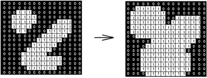
G. Morphological Process
1) Erosion And Dilation: The2erosion2of2a2binary2image2f 2by2a2structuring2element2s2(denoted f
s)2produces2a2new2binary2image g = f s with2ones2in2all2locations2(x,y) of a2structuring2element's2origin
at2which2that2structuring2element s2fits2the2input2image f, i.e. g(x,y) = 1 is s2fits f and
02otherwise,2repeating2for2all2pixel2coordinates (x,y).
Erosion2with2small (e.g. 2×2 - 5×5)2square2structuring2elements2shrinks2an2image2by2stripping2away2a2layer2of2pixels
from2both2the2inner2and2outer2boundaries2of2regions. 2The2holes2and2gaps2between2different2regions2become2larger,
Fig. 3.3 Erosion: 3×3 square structuring element
Larger2structuring2elements2have a2more2pronounced2effect,2the2result of2erosion2with a2large2structuring
element2being2similar2to2the2result2obtained2by2iterated2erosion2using a2smaller2structuring2element2of2the2same2shape. If s1
and s2 are a2pair2of2structuring2elements2identical2in2shape,with s22twice2the2size of s1, then f s2≈ (f s1) s1.
Erosion removes small-scale details from interested image by2subtracting2the2eroded2image2from2the2original2image,
boundaries2of2each2region2can2be2found: b = f − (f s ) where f is an2image2of the2regions, s is a 3×3 structuring2element, and b
is an2image2of2the2region2boundaries.
The2dilation2of2an2image f by a2structuring2element s (denoted f s)2produces a2new2binary2image g = f s
with2ones2in2all2locations (x, y) of a2structuring2element's2orogin2at2which2that2structuring2element2s2hits2the2the2input
image f, i.e. g(x, y) = 1 if s hits f and 0 otherwise,2repeating2for2all2pixel2coordinates (x, y). Dilation2has2the2opposite2effect
to2erosion – it2adds a2layer2of2pixels2to2both2the2inner2and2outer2boundaries2of2regions.
The2holes2enclosed2by2a2single2region2and2gaps2between2different2regions2become2smaller,2and2small
intrusions2into2boundaries2of2a2region2are2filled2in:
Fig. 3.4 Dilation: a 3×3 square structuring element
Results2of2dilation2or2erosion2are2influenced2both2by2the2size2and2shape2of2a2structuring2element.
Dilation2and2erosion2are2dual2operations2in2that2they2have2opposite2effects. Let f c denote2the2complement2of2an2image f,
i.e., the2image2produced2by2replacing 1 with 0 and2vice2versa. Formally, 2the2duality2is2written2as
f s = f csrot
where srot is2the2structuring2element2s2rotated2by 180. If2a2structuring2element2is2symmetrical2with2respect2to rotation, then
srot does2not2differ2from s. If2a2binary2image is2considered2to2be2a2collection2of2connected2regions2of pixels2set to 1
on2a2background2of2pixels2set to 0, then2erosion is2the2fitting2of a2structuring2element2to2these2regions
and2dilation2is2the2fitting2of2a2structuring2element2(rotated2if2necessary)2into2the2background, followed2by2inversion2of
the2result.
[image:6.612.106.506.415.566.2]The test of projected technique to discover and segment brain tumor is performed using MR images. Each tested image has brain tumor of diverse intensity, size and shape. Manual examination is done to check the correctness of automatically segmented tumor area. The experimental result for MR images containing tumor is discussed below.
[image:7.612.59.558.467.599.2]’ Fig. 4.1 Input MRI image Fig. 4.2 Trilateral filtered image
Fig. 4.3 Filtred input for EM-GM Segmentation Fig 4.4 EM-GM segmented image
In Fig 4.1, it is one of the MRI image containing tumor which is taken as the input. Fig 4.2 shows the resultant image after the Trilateral filtering process. Fig 4.3 shows the filtered input image for EM-GM Segmentation and the Fig 4.4 shows the resultant image of EM-GM Segmentation.
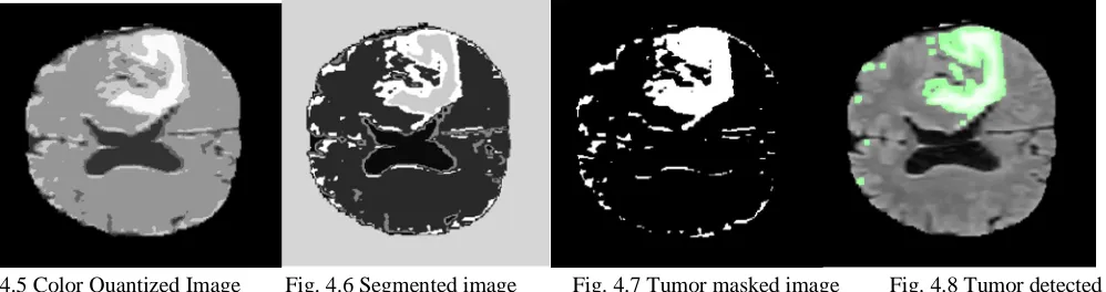
Fig. 4.5 Color Quantized Image Fig. 4.6 Segmented image Fig. 4.7 Tumor masked image Fig. 4.8 Tumor detected
After the EM-GM Segmentation the resultant image is color quantized, this is shown in the Fig 4.5. Later we will train the SOM (Self-organizing map) which is a type of artificial neural network. It is trained using unsupervised learning to produce a two dimensional discretized representation of the input space of the training samples. Fig 4.6 shows us the Classified and Segmented image which is done after the color quantization process. After the Segmentation process the tumor will be masked and the Fig 4.7 shows the resultant image of the tumor masked region/area. Morphological cleaning is done after masking the tumor and the final stage is tumor detection which is shown in the resultant image Fig 4.8, the region which is highlighted by green colour shows us the presence of tumor in the MR image.
V. CONCLUSION AND FUTURE WORK
classifier and spotting of tumor was done with image segmentation. Pattern recognition was performed using probabilistic neural network with radial basis function and pattern will be characterized with the help of fast discrete curvelet transform and haralick features analysis. Here. Spatial fuzzy clustering algorithm was utilized effectively for accurate tumor detection to measure the area of abnormal region. From an experiment, system proved that it provides better classification accuracy with various stages of test samples and it consumed less time for process.
REFERENCES
[1] N. Kwak, and C. H. Choi, “Input Feature Selection for Classification Problems”, IEEE Transactions on Neural Networks, 13(1), 143–159, 2002.
[2] E. D. Ubeyli and I. Guler, “Feature Extraction from Doppler Ultrasound Signals for Automated Diagnostic Systems”, Computers in Biology and Medicine, 35(9), 735–764, 2005.
[3] D.F. Specht, “Probabilistic Neural Networks for Classification, mapping, or associative memory”, Proceedings of IEEE International Conference on Neural Networks, Vol.1, IEEE Press, New York, pp. 525-532, June 1988.
[4] D.F. Speech, “Probabilistic Neural Networks” Neural Networks, vol. 3, No.1, pp. 109-118, 1990.
[5] Georgia is. Et all , “ Improving brain tumor characterization on MRI by probabilistic neural networks and non-linear transformation of textural features”, Computer Methods and program in biomedicine, vol 89, pp24-32, 2008
[6] Klaus M., “Automated segmentation of MRI brain tumors”, Journal of Radiology ,vol. 218, pp. 585-591,2001
[7] Kernel, P., Bela, M., Rainer, S., Zalan, D., Zsolt, T. and Janos, F., “Application of neural network in medicine”, Diag. Med. Tech.,vol. 4,issue 3,pp: 538-54 ,1998.
[8] Mammadagha Mammadov, Engin tas , “An improved version of back propagation algorithm with effective dynamic learning rate and momentum” Inter Conference on Applied Mathematics ,pp:356-361, 2006.