6
I
January 2018
Net benefit evaluation method for solar tracker
connected PV systems
Cristina Cabo Landeira1, Ángeles López-Agüera2 1, 2
Sustainable Energetic Applications Group, Faculty of Physics, Santiago de Compostela University
Abstract: A wide percentage of the current PV systems use tracker as system’s design, especially in developed countries. However, this election is not a consequence of an exhaustive evaluation. On this paper, a method to evaluate the suitability of a tracker compared to a fixed-tilt PV system is presented. The best compromise between power production, lifecycle analysis and economic costs are taken into account during the analysis. The used lifecycle estimators are the energy payback time for the Lifecycle Analysis and the Internal Rate of Return for the economic investment. Experimentally-validated meteorological data from NASA-SSE service have been used. The solar tracker system net gain is evaluated in terms of diffuse radiation component fraction. As final result, a net gain map for primarily evaluate the benefit of installing a tracker compared to a fixed-tilt PV system for each Köppen-Geiger climate types is presented. The proposed method allows making the right design decision for future installations. This is especially relevant for developing countries, with the highest PV market growing perspective.
Keywords: PV system; solar tracker; PV design; Tracker net gain; Köppen
I. INTRODUCTION
Solar photovoltaic is, nowadays, considered as one of the most promising renewable energy sources [1]. Currently, the 25% of the operating PV systems are equipped with solar tracking system [2][3]. The trackers market share is expected to keep growing over 5% per year during the next decade [4].
However, the trackers market deployment is not result of a detailed evaluation of its suitability. Currently, in terms of net power production increase, there is no a general criterion to primarily assess its adequateness for any globe location. It is generally assumed that installing solar trackers boost the collected energy by following the sun’s path. Even if a large number of papers analyse solar trackers, no conclusions can be extracted as no systematic studies have been carried out. Several researches establish the production increase percentage between 10%-45% when installing a tracker system. Although while some studies considered location-dependent data [5][6][7], others are microphysics model-dependent [8][9][10].
In addition, the power production increase is not enough to determine the advantages of including a solar tracker on a PV system design. The suitability assessment requires to consider both environmental and economic associated costs [11][12].
A recent study evaluates the solar tracker suitability, leading to promising results [13]. By developing an algorithm based on experimental, non-model dependent data, the production increase of a solar tracker compared to a fixed-tilt system can be calculated. This is done as function of the daily diffuse fraction values and is tested on a medium-irradiation region. The innovative feature is that this method calculates the solar tracker net increase after considering the power production and the associated costs. Using these results, this paper aims to create a net benefit solar tracker criterion to evaluate its installation suitability.
To ensure a worldwide validity, a global data source with solar radiation values and a climate classification has been performed. As a hypothesis, the net gain results for daily diffuse fraction will be used with the monthly average radiation values. For the climate data, the NASA-SSE quasi-experimental meteorological database is selected as it provides diffuse radiation values. The retrieved values will be validated with experimental solar radiation data [14]. Besides, the statistical uncertainties will be considered on the final results. For the classification, the Köppen-Geiger climate classification will be used by retrieving statistical data for each climate considering similarity criterion [15].
As final result, a worldwide map showing the net gain for each Köppen-Geiger climate is presented. The proposed method allows to make the right design decision for future installations. This is especially relevant for developing countries, with the highest PV market growing perspective.
II. METHODOLOGY
climatic variable: the percentage of diffuse component on the global solar radiation. Applying the proposed procedure should be simple if a dedicated irradiation database was available for any PV system location of interest. Unfortunately, more than 80% of the globe suffers from a deep lack of experimental irradiation data.
To palliate the insufficiency of meteorological stations with historical data records around the planet, the use of the NASA-SSE meteorological database is proposed [14]. These data, particularly the diffuse radiation values, are generated after mathematical models. To validate the model, AEMET experimental data have been considered [16][17].
Following the Köppen-Geiger methodology [15], each selected planet location is classified to generalize the results. The classification will be characterized in terms of diffuse fraction using the previously validated NASA database.
A. Climate classification
The Köppen-Geiger climate classification is selected for the analysis as it requires only of precipitation and temperature data [15][18]. Therefore, it is independent of the solar irradiation levels or other parameters. This eases the climate characterization in locations where no data historic is available. By using up to three letters, the climate is described on its general type (1st letter, Table 1), precipitation level (2nd letter) and temperature range (3rd).
TABLE 1
Main Köppen-Geiger climate groups
Group Climate type
A Tropical
B Desert and semi-arid
C Temperate
D Continental
E Polar
B. Global and diffuse data source
The creation of a large enough database to characterize different climates requires to find a data source with worldwide meteorological data. The NASA-SSE (Surface meteorology and Solar Energy) database is selected as it has 23 years of monthly mean meteorological values for any latitude-longitude pair [19]. This dataset is based on the Pinker and Laszlo shortwave algorithm with an effective 30x30 km pixel size. The dataset refers a RMSE of 8.71% for global horizontal and 22.78% for diffuse horizontal irradiances [20]. The high uncertainty related to the applied model requires its validation with an experimental data source.
To cross-check the solar radiation data precision, the Spain’s State Meteorological Agency AEMET database is considered [16]. The AEMET experimental dataset, with 29 meteorological stations, is compared with the CM-SAF (Climate Monitoring Satellite Application Facilities) satellite data. This dataset has a high resolution (3x3 km) and high accuracy (0.19 kWh/m2day maximum deviation with respect to data from 12 meteorological stations around the world). A 6.7% difference between both databases is observed. This ensures the validity of AEMET database.
Global and diffuse radiation annual average values for 47 Spanish cities from AEMET and NASA-SSE are compared to validate the NASA database reliability [17]. Table 2 shows the difference between both data sources in terms of global and diffuse radiation, as well as diffuse fraction. The low difference between both datasets allows to consider the NASA-SSE solar radiation values as valid.
TABLE 2
Difference of annual average NASA radiation values with the AEMET data source for validation Global radiation Diffuse radiation Diffuse Fraction
-8.01% -6.2% -2.87%
C. Data sample selection
Once the solar radiation, temperature and precipitation data source is defined, the locations for data gathering must be selected [21]. With the aim of characterize the different climates in detail, over 40 000 values from nearly 800 inhabited cities around the world are initially selected. Gathered values for each location include:
Temperature, precipitation and global plus monthly diffuse radiation.
To ensure as much as possible an unbiased database, some constraints are applied during each Köppen-Geiger climate types subsample selection process. So, the accepted variation range, in latitude and longitude, is 0.5º inside each subsample. In addition, a similarity altitude criterion is applied.
A final sample of 35 000 values from almost 700 cities belonging to 29 Köppen-Geiger climates are obtained. For each value, diffuse fraction is calculated for further analysis.
D. Diffuse fraction pattern of behaviour definition for Köppen-Geiger climate classification
By using the database defined on Section 2.C, subsamples for each of the 29 Köppen climatic regions are considered. For each subsample, the monthly average fraction of diffuse radiation component, DF, and its standard deviation are calculated. The DF is defined as the ratio between the diffuse and global irradiation values, both in a monthly basis. Table 3 resumes the available dataset for each general climate type and the obtained statistical reliability. As previously explained, restrictions in terms of height above sea level are applied to ensure sample similarity.
a) b)
c) d)
[image:4.612.96.515.230.701.2]e)
TABLE 3
Available statistic and data analysis results for each Köppen-Geiger climate
Köppen climate
Sample statistic
Data inside the interval
σ 2σ
A 131 67.00% 96.21%
B 114 68.25% 96.48%
C 227 71.91% 97.62%
D 184 75.07% 97.18%
[image:4.612.313.503.239.470.2]E 33 67.05% 97.54%
Figure 1 shows the average diffuse fraction patterns for each of the 29 climate types. After the statistical analysis, it can be
determined that, in average, 97% of the monthly values lie inside the 2σ interval. This ensures the representativeness of the
performed characterization, where each climate shows a specific pattern.
III.RESULTS
Recent studies found a linear relationship between climatic conditions and the benefit of a tracker design with respect to a fixed-tilt PV system [13]. For this relation, the climatic conditions representative variable is the Diffuse Fraction, DF, as previously define. Two different benefit parameters are considered: The Production Benefit, associated only to power production, and the Net Benefit, where economic and environment costs are also considered. In the following, the proposed methods will be applied to characterize each Köppen-Geiger climate in terms of both production and net benefits.
[image:5.612.149.468.289.457.2]The DF worldwide database built in the previous section constitutes the analysis basis. Even if the monthly characterization computed above is useful for different sizing procedures and PV installation analyses [22], it overcomes the required detail for the current work. For this purpose, only annual values will be used. Figure 2 shows the annual Diffuse Fraction average, <DF>Annual, for each climate. It must be notice that associated error for Dsc and EF climates is due to the difficulty of gathering statistic in extreme climates (subarctic and polar respectively). The standard error shows an average value of 4.1%. This low error value ensures the validity of the gathered data for the intended analysis and climate characterization.
Figure 2. Annual diffuse fraction average value for each Köppen-Geiger climate type
A. Power production benefit
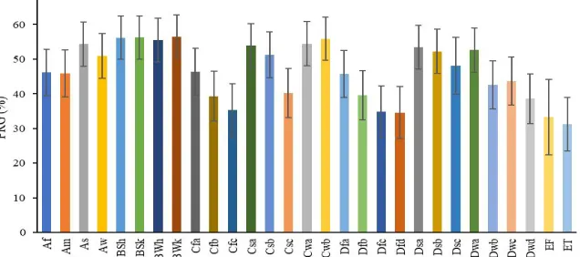
The production benefit (in %) of a solar tracker compared to a fixed-tilt PV is measured in terms of Performance Ratio Gain, PRG. Following the experimental data analysis performed in [13], the PRG shows a direct linear shape with the diffuse fraction. The main characteristics are a slope of (-78.72 ±8.38) and an intercept of (79.75±5.62). By applying this linear fit to each climate’s average annual diffuse fraction, the PRG variation per climate is obtained. Results are plotted in Figure 3, including the computed associated uncertainty. As total average, the tracker system performs 46.5% better than the fixed tilt one with a 7% standard error.
[image:5.612.151.469.578.719.2]B. Net benefit
To evaluate the net benefit of a solar tracker with respect to a fixed-tilt PV system, the Performance Ratio Net Gain, PRNG, is used. It is defined as the convolution of the performance ratio gain, PRG, and the Overall Associated Costs, OAC, which includes both economic and environmental costs [13]. The economic expenses associated to the PV system are measured with the Internal Rate of Return. These expenses are related with the solar tracker purchase and maintenance. The environmental cost is correlated to the Energy Payback Return Time, defined as the required operation time to produce the energy consumed in the production, construction plus functioning. As in the previous case, the PRNG shows a linear behaviour with the diffuse fraction, as written in Eq. 1.
PRNG = (−78.72 ± 8.38)DF + (32.10 ± 9.96) (%) Eq. 1
By applying this linear fit to each climate <DF>Annual, the corresponding PRNG is obtained. Figure 4 shows the performance ratio net gain (in %) of a tracker-equipped compared to a fixed tilt system for each Köppen-Geiger climate after each annual average diffuse fraction.
[image:6.612.110.509.315.552.2]Climates with positive PR net gain are divided into regions with an average net gain under 5% (scenarios with operating benefit for installing a tracker, marked in green) and over 5% (highly profitable tracker installation, in orange). Anyhow, it must be noticed that these are direct production increases as all the expenses related with the tracker installation are included. From the corresponding statistical analysis an average 11% standard error was obtained.
Figure 4.Performance ratio net gain after average annual diffuse fraction values for each Köppen-Geiger climate once considered the overall costs (with standard errors)
Thus, from the results and considering the large analysis-associated uncertainties, some additional remarks about the net gain can be obtained. For that, three different categories will be defined:
1) Totally not advised climates: The full PRNG obtained interval moves in the negative range. A fixed tilt PV system is particularly suggested on these climates.
2) Positive tendency climates: For these climates, the PRNG is mainly on the positive range, even if negative values are possible. For this reason, positive tendency is adequate instead of referring to totally positive climates.
3) No conclusive climates: The PRNG results move along a positive to negative data range. Design decision-making requires a higher data statistic or on-location experimental data.
The full procedure is based on the average annual diffuse fraction values. Just by knowing the location’s climate classification, the Köppen-Geiger classification average values can be used. As an added value, these results can be used for specific locations where historical records of solar global and diffuse values are available. Using solar radiation experimental data will allow to obtain more accurate results.
TABLE 4
Köppen-Geiger climates solar tracker net gain results
Köppen-Geiger climate classification
Performance Ratio
Net Gain interval (%) Result
Maximum Minimum
Tropical rainforest Af 9,11 -12,15 No conclusive
Tropical monsoon Am 8,85 -12,43 No conclusive
Savannah As 17,09 -3,70 Positive tendency
Tropical wet Aw 13,73 -7,17 Positive tendency
Hot semi-arid BSh 18,84 -1,79 Positive tendency
Cold semi-arid BSk 18,90 -1,72 Positive tendency
Hot desert BWh 18,16 -2,53 Positive tendency
Cold desert BWk 19,18 -1,46 Positive tendency
Humid subtropical Cfa 9,34 -11,90 No conclusive
Temperate oceanic Cfb 2,56 -19,23 Totally not advised
Subpolar Cfc -1,19 -23,52 Totally not advised
Hot-summer Mediterranean Csa 16,61 -4,11 Positive tendency
Warm-summer Mediterranean Csb 14,10 -6,98 Positive tendency
Cool-summer Mediterranean Csc 3,38 -18,26 Totally not advised
Monsoon-influenced humid subtropical Cwa 17,22 -3,58 Positive tendency
Subtropical highland Cwb 18,57 -2,10 Positive tendency
Hot-summer humid continental Dfa 8,66 -12,64 No conclusive
Warm-summer humid continental Dfb 2,79 -18,95 Totally not advised
Subarctic Dfc -1,72 -23,88 Totally not advised
Extremely cold subarctic Dfd -1,89 -24,18 Totally not advised
Hot, dry-summer continental Dsa 16,14 -4,61 Positive tendency
Warm, dry-summer continental Dsb 15,03 -5,83 Positive tendency
Dry-summer subarctic Dsc 12,02 -11,15 Positive tendency
Monsoon-influenced hot-summer humid Dwa 15,36 -5,47 Positive tendency
Monsoon-influenced warm-summer humid
continental Dwb 5,64 -15,87 No conclusive
Monsoon-influenced subarctic Dwc 6,76 -14,78 No conclusive
Monsoon-influenced extremely cold
subarctic-continental Dwd 1,83 -19,94 Totally not advised
Tundra EF -0,75 -28,06 Totally not advised
Ice cap ET -5,14 -27,71 Totally not advised
C. Solar tracker net gain map
As visualization of the previous results, Figure 5 shows the net benefit of installing a solar tracker. For this map, the performance ratio net gain results after Table 4 have been considered.
Moreover, the existence of areas with microclimates can affect to the net improvement estimation. Therefore, a location’s climatic study is recommended to ensure the data reliability.
Europe (except Balkans Peninsula, Central/Southern Iberian Peninsula and Italy). Some of these non-advised regions currently have a wide solar tracker presence. Nowadays, trackers global market is dominated by Europe (almost a 40% of the market share) with the highest demands from Italy, Spain and Germany [3]. Germany, with mainly Cfb and Dfa climates, is an example of not advised to not conclusive location. By applying a conservative criterion, fixed-tilt systems are preferable than solar tracker systems. Even so, it is the third European market for these systems.
Figure 5. World solar tracker net gain
IV.CONCLUSIONS
This paper aims to develop a method to evaluate the associated net power production increase of installing a solar tracker compared to a fixed-tilt system design. For this purpose, the production benefit of a tracker versus a fixed system will be assessed as a climate function.
The calculation is performed after an experimental algorithm which takes into consideration the solar tracker associated costs: The EPBT (the consumed energy for manufacturing the tracker), the economic investment (for the tracker acquisition and maintenance) and the solar tracker system energy consumption.
To extend the results to any globe location, a relation between solar radiation and The Köppen-Geiger climate classification is developed. For that, a database for each climate type is built and the diffuse fraction curves are plotted. The statistical analysis
results show a 97% of the values inside the 2σ interval, ensuring its representativeness.
Without considering the overall associated cost, a solar tracker performs a 46.5% better than a fixed-tilt system in annual average. Once considering the OAC, a linear relation algorithm between the Performance Ratio Net Gain and the Diffuse Fraction is obtained. Applying this relation to each annual average diffuse fraction value, the Net Gain intervals for each climate can be determined. The results analysis shows three different scenarios depending on the values range. For nine climates, the results lead to not advise the tracker installation. These climates are mainly humid and frequent on latitudes above 40ºN. Some of these non-advised regions are currently regions with a wide solar tracker presence. As an example, Europe is the main market for the trackers PV systems, even if only the southern regions can be considered adequate.
Fourteen climates show a positive tendency for the net gain. These climates mainly are tropical savannah, steppes and deserts. Also, Mediterranean climates (including continental, hemi-boreal and subtropical highland) show direct benefit, as well as some oceanic, subpolar (dry and temperate summer) and continental (dry winter) climates seem optimal for installing solar tracking systems. For the remaining six climates, the method does not provide a conclusive result. Making a proper decision on the system design will require a greater statistics or on-location experimental data.
Besides, a world map for results general visualization is presented.
REFERENCES
[1] IEA (International Energy Agency), “Snapshot of Global Photovoltaic Markets - IEA PVPS,” 2017.
[2] Global Market Insights, “Solar PV Mounting Systems Market worth $9bn by 2024: Global Market Insights, Inc.,” 2017. [Online]. Available: https://globenewswire.com/news-release/2017/05/25/995994/0/en/Solar-PV-Mounting-Systems-Market-worth-9bn-by-2024-Global-Market-Insights-Inc.html. [Accessed: 10-Jan-2018].
[3] Global Market Insights, “Global Solar Tracker Market Size will reach USD 6.37 Billion by 2020.” [Online]. Available: https://globenewswire.com/news-release/2017/06/01/1005367/0/en/Global-Solar-Tracker-Market-Size-will-reach-USD-6-37-Billion-by-2020.html. [Accessed: 10-Jan-2018].
[4] S. Moskowitz, “The Global PV Tracker Landscape 2016 : Prices , Forecasts , Market Shares and Vendor Profiles Table of Contents List of Figures,” 2016. [5] S. Seme et al., “Dual-axis photovoltaic tracking system – Design and experimental investigation,” Energy, pp. 1–8, 2017.
[6] H. Fathabadi, “Comparative study between two novel sensorless and sensor based dual-axis solar trackers,” Sol. Energy, vol. 138, pp. 67–76, 2016.
[7] A. Öztürk, S. Alkan, U. Hasirci, and S. Tosun, “Experimental performance comparison of a 2-axis sun tracking system with fixed system under the climatic conditions of Düzce, Turkey,” Turkish J. Electr. Eng. Comput. Sci., vol. 24, no. 5, pp. 4383–4390, 2016.
[8] A. Bahrami, C. O. Okoye, and U. Atikol, “Technical and economic assessment of fixed, single and dual-axis tracking PV panels in low latitude countries,” Renew. Energy, vol. 113, pp. 563–579, 2017.
[9] M. De Simón-Martín, C. Alonso-Tristán, and M. Díez-Mediavilla, “Sun-trackers profitability analysis in Spain,” Prog. Photovolt Res. Appl., vol. 22, no. February 2013, pp. 1010–1022, 2013.
[10] A. Bahrami, C. O. Okoye, and U. Atikol, “The effect of latitude on the performance of different solar trackers in Europe and Africa,” Appl. Energy, vol. 177, pp. 896–906, 2016.
[11] R. Fu et al., “U.S. Solar Photovoltaic System Cost Benchmark: Q1 2016,” Natl. Renew. Energy Lab., no. September, p. 37, 2016.
[12] M. García, J. A. Vera, L. Marroyo, E. Lorenzo, and Miguel Pérez, “Solar-tracking PV Plants in Navarra: A 10 MW Assessment,” Prog. Photovolt Res. Appl., vol. 17, no. April 2009, pp. 337–346, 2009.
[13] C. Cabo Landeira and Á. López-Agüera, “PV Tracker System Net Gain Associated o the Local Climatic Conditions,” Int. J. Res. Appl. Sci. Eng. Technol., vol. 6, no. I, pp. 185–193, 2018.
[14] “NASA SSE: Surface meteorology and Solar Energy.” [Online]. Available: https://eosweb.larc.nasa.gov/sse/. [Accessed:
[15] M. Kottek, J. Grieser, C. Beck, B. Rudolf, and F. Rubel, “World map of the Köppen-Geiger climate classification updated,” Meteorol. Zeitschrift, vol. 15, no. 3, pp. 259–263, 2006.
[16] “Agencia Estatal de Meteorología - AEMET. Gobierno de España.”
[17] Sancho, J. Riesco, and C. Jiménez, Atlas de Radiación Solar en España. Ministerio de Agricultura, Alimentación y Medio Ambiente, 2012.
[18] D. Chen and H. W. Chen, “Using the Köppen classification to quantify climate variation and change: An example for 1901–2010,” Environ. Dev., vol. 6, pp. 69–79, Apr. 2013.
[19] “NASA Surface meteorology and Solar Energy - Available Tables.” [Online]. Available: https://eosweb.larc.nasa.gov/cgi-
bin/sse/grid.cgi?&num=091106&lat=15.173&submit=Submit&hgt=100&veg=17&sitelev=-999&[email protected]&p=grid_id&p=srf_alb&step=2&lon=-89.986. [Accessed: 04-Sep-2015].
[20] M. Sengupta et al., “Best Practices Handbook for the Collection and Use of Solar Resource Data for Solar Energy Applications,” 2015. [21] “Weatherbase - Travel Weather Averages.” [Online]. Available: http://www.weatherbase.com/. [Accessed: 07-Dec-2017].
[22] F. Núñez Sánchez and Á. López-Agüera, “Optimización do proceso de dimensionamento en instalacións fotovoltaicas illadas empregando un algoritmo de probabilidade de perda de carga ( LLP ),” Trab. Fin Grado. Fac. Física. Univ. Santiago Compost., p. 33, 2017.