Optimization of Surface Roughness and Kerf
Width Parameters in Wire Cut EDM Process
through Response Surface Methodology.
A. Damodara Reddy1
1
Assistant Professor, Mechanical Engineering Department, JNTUA College of Engineering, Pulivendula.
Abstract: Machining of Composite materials like Al 7075-SiC metal matrix composites has found its use extensively in Air craft fittings, gears, shafts, missile parts, regulating valve parts, keys and bike frames to enhance high strength, corrosion resistance and thermal resistance characteristics. And also there is a need to improve high material removal rate, better surface finish and good dimensional accuracy. Conventional machining is not able to satisfy these demands. Wire electro discharge machining plays a major role in machining of conductive materials with intricate shapes and complex geometries where a thin metallic wire of 0.1-0.3mm diameter is used as a tool electrode. Al 7075-SiC metal matrix composites are prepared by using Sand casting though manual stirring. The objective is to identify the best parametric combination of Wire EDM to minimize surface roughness and kerf width for Al 7075-10% SiC and Al 7075-15% SiC. For this experimentation Pulse on time(TON), pulse off time(TOFF), peak current(IP) and Spark gap Voltage are the most affecting input parameters to perform experiments on Wire Cut Electro Discharge Machine(ELPULSE 40A). In the present work 34 experimental runs are designed based on the Box-Behnken Design of Response Surface Methodology. ANOVA (Analysis of Variance) is used to get the effect of process parameters on process response. A second order polynomial model has been developed to correlate the process responses and the machining parameters by using Response Surface Method (RSM).
Keywords: Include at least 5 keywords or phrases
I. INTRODUCTION
Wire Cut Electro Discharge Machining is an unconventional Electro Thermal machining process which is working based on the principle of repetitive sparking cycles. Due to generation of heat melting and evaporation of both wire and work piece takes place. Gap between wire and work piece is in range of 0.025-0.5mm which is maintained constant by computer controlled positioning system. The gap between wire and work piece is covered with steam of dielectric fluid which is directed to the working zone by the nozzles present at the upper and lower diamond guides. The dielectric can control sparking, cools the process and flushes away the tiny particles very faster. The wire and work piece is mounted on CNC work table. Wire is fed through work piece by a microprocessor to enable machining.
The wire EDM can cut almost all the metals including aluminium, copper, carbide, graphite, steel and titanium. Depending upon the hardness of work piece wire metal changes. With the advent of WEDM process a path provided by CNC is used to machine hard metals through inaccessible locations with the use of electrical sparks exist between tool and work piece. Al most all the areas like aerospace, semiconductor, tool and die making industries are now a days using Wire cut EDM process.
With the increase in demand for high hard, light weight and temperature resistant materials in aerospace, automobile and missile applications quality of a product has became a major concern. And also minimizing of material wastage during machining is important. Wire cut Electro Discharge Machining is the best choice to achieve all these requirements. The present study deals with identification of the best parametric combination of a Wire cut EDM process parameters to achieve minimum surface roughness and kerf width. By using ANOVA the effect of process parameters on process responses has been found.
II. EXPERIMENTALDETAILS
A. Response Surface Methodology
Response Surface Methodology is a collection of mathematical and statistical techniques useful for modeling and analysis of a problem in where the responses of interest is influenced by several variables and objective is to optimize this response. An optimal response can be obtained by choosing a proper choice of design and operating conditions on a set of controllable variables. Here output is influenced by the number of input factors. In this method the main goal is, to reduce the expensive analysis cost and optimize the output responses that are influenced by various input parameters. For the visualization of the response, contour and surface plots are used. It gives the relation between the control factors and output responses. Contour plots are used to visualize the shape of response surface.
Suppose ‘x1' and ‘x2’ are the input parameters that are affecting the response ‘y’ can be expressed as follows: y=f(x1,x2)+Ɛ(a)
where Ɛ is the noise or error observed in response ‘y’
Let E(y) = f(x1,x2) = η (b)
The above experiment is the expected response which is known as response surface with levels of ‘x1’ and ‘x2’. RSM comprises the following steps
1) Prepare a set of trials for sufficient and consistent extent of the output.
2) Progress an empirical model of the 2nd order response surface with the suitable sets.
3) Identify the efficient set of trial variables that gives a maximum and minimum response values.
4) Characterize the direct and the collaborative effects of variables through 2D and 3D graphs.
B. Plan of Experiments
Very vital stage of RSM is to progress a set of trials later difficult detection. Engineering exploration problems are practical in nature and include use of practice.
There are various designs like
1) Box Behnken Design
2) Full factorial
3) Fractional factorial (FFD)
4) One factor
5) D- optimal
6) Latin square
7) CCD
8) Historical data
C. Design of Experiments – Box Behnken Design
Process Parameters Units Level 1 Level 2 Level 3
Pulse on time (A) Micro sec 100 105 110 Pulseoff time(B) Micro sec 59 60 61 Peak Current(C) Amphere 180 190 200 Sparkgap Voltage(D) Volts 10 15 20
Table 1 Process parameters and their limits
Such a way that the estimation of the regression parameters for the factor effects are not affected by the blocks. In other words, in these designs the block effects are orthogonal to the other factor effects. Yet another advantage of these designs is that there are no runs where all factors are at either the +1 or -1 levels. This could be advantageous when the corner points represent runs that are expensive or inconvenient because they lie at the end of the range of the factor levels.
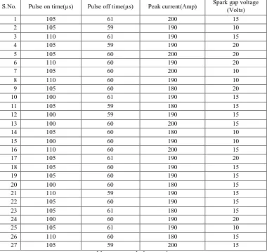
S.No. Pulse on time(µs) Pulse off time(µs) Peak current(Amp) Spark gap voltage (Volts)
1 105 61 200 15
2 105 59 190 10
3 110 61 190 15
4 105 59 190 20
5 105 60 200 20
6 110 60 190 20
7 105 60 200 10
8 110 60 190 10
9 105 60 180 20
10 100 61 190 15
11 105 59 180 15
12 100 59 190 15
13 100 60 200 15
14 105 60 180 10
15 100 60 190 10
16 110 60 200 15
17 105 61 190 20
18 105 60 190 15
19 105 60 190 15
20 100 60 180 15
21 110 59 190 15
22 105 60 190 15
23 105 61 180 15
24 100 60 190 20
25 105 61 190 10
26 110 60 180 15
[image:4.612.118.498.231.590.2]27 105 59 200 15
Table 2: Box-Behnken Design
D. Selection of Material
Al 7075- SiC Metal Matrix Composites with varying composition of 10% and 15% Silicon Carbide are used for the melting temperature that is 650OC. And then Silicon Carbide particle of size 50 microns is added into the matrix alloy according to the proportion. This combination has to be stirred for some time and then poured into the previously prepared sand mould.
Material Weight of Al 7075(gm)
Weight of SiC(gm)
Rockwell Hardness
Al 7075- 10%SiC 1800 200 120.67 Al 7075- 15%SiC 1700 300 183.33
Fig 2. Al 7075-SiC(10% and15%) after casting
III.RESULTSANDDISCUSSIONS
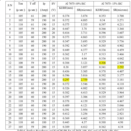
The experiments are performed based on the order of Box-Behnken Design and responses characteristics like Surface Roughness and Kerf Width have been observed by using Talysurf and Tool makers microscope are tabulated below
A. Response Table for Surface Roughness and Kerf Width
S.N o
Ton T off Ip SV Al 7075-10% SiC Al 7075- 15% SiC
(μ sec ) (μ sec ) (Amp) (V) KERF(mm)
SR(microns) KERF(mm) SR(microns)
1 105 61 200 15 0.374 3.874 0.353 3.708
2 105 59 190 10 0.372 4.085 0.34 3.271
3 110 61 190 15 0.375 5.335 0.397 4.211
4 105 59 190 20 0.447 3.78 0.366 3.368
5 105 60 200 20 0.416 3.711 0.396 3.607
6 110 60 190 20 0.373 4.863 0.333 6.041
7 105 60 200 10 0.347 3.693 0.329 3.736
8 110 60 190 10 0.392 4.367 0.385 4.902
9 105 60 180 20 0.449 4.377 0.336 4.459
10 100 61 190 15 0.362 3.17 0.313 3.466
11 105 59 180 15 0.381 4.04 0.336 4.042
12 100 59 190 15 0.384 3.121 0.306 2.909
13 100 60 200 15 0.38 3.057 0.341 2.292
14 105 60 180 10 0.436 3.305 0.378 4.407
15 100 60 190 10 0.396 3.016 0.392 3.177
16 110 60 200 15 0.297 2.759 0.388 3.181
17 105 61 190 20 0.372 3.546 0.391 4.118
18 105 60 190 15 0.326 4.802 0.362 4.063
19 105 60 190 15 0.382 4.413 0.329 3.964
20 100 60 180 15 0.397 3.306 0.335 3.087
21 110 59 190 15 0.378 4.139 0.315 4.467
22 105 60 190 15 0.409 4.121 0.339 5.046
23 105 61 180 15 0.391 3.954 0.369 3.675
24 100 60 190 20 0.412 3.256 0.394 2.921
25 105 61 190 10 0.369 4.462 0.371 3.863
26 110 60 180 15 0.443 4.37 0.388 4.98
27 105 59 200 15 0.389 4.412 0.362 4.34
B. Analysis of Variance and Regression Equations
Source Sum of
Squares df
Mean
Square F-Value
p-value
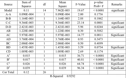
Prob> F Remarks Model 0.11 14 7.962E-003 19.67 < 0.0001 significant
A-A 8.090E-004 1 8.090E-004 2.00 0.1736 B-B 1.164E-003 1 1.164E-003 2.88 0.1062
C-C 9.366E-003 1 9.366E-003 23.14 0.0001 significant D-D 2.421E-003 1 2.421E-003 5.98 0.0244 significant
AB 1.228E-004 1 1.228E-004 0.30 0.5882
AC 5.978E-003 1 5.978E-003 14.77 0.0011 Significant AD 3.760E-004 1 3.760E-004 0.93 0.3473
BC 2.006E-004 1 2.006E-004 0.50 0.4899
BD 1.453E-003 1 1.453E-003 3.59 0.0734 Significant CD 1.089E-003 1 1.089E-003 2.69 0.1174
A2 0.015 1 0.015 36.71 < 0.0001 Significant B2 0.017 1 0.017 40.81 < 0.0001 Significant C2 0.026 1 0.026 64.74 < 0.0001 Significant D2 0.039 1 0.039 96.34 < 0.0001 Significant Cor Total 0.12 26
R-Squared 0.9292
Table5. ANOVA Table for Kerf Width on machining of Al 7075-10%SiC
C. Regression Equation for Kerf Width
143.12942-0.21847*Ton-4.12600*Toff-0.084458*Ip+0.13222*SV+9.50000E-004*Ton*Toff-6.45000E-004*Ton*Ip-3.50000E-004*Ton*SV-6.25000E-004*Toff*Ip-3.60000E-003*Toff*SV+2.80000E-004*Ip*SV+ 1.37167 E-003*Ton2+0.034917*Toff2 +4.81667E-004* Ip2+2.33167E-003*SV2.
Source Sum of
Squares df
Mean
Square F-Value
p-value
Prob> F Remarks
Model 13.16 14 0.94 6.19 0.0002 Significant
A-A 2.01 1 2.01 13.21 0.0018 Significant
B-B 0.13 1 0.13 0.84 0.3714
C-C 0.28 1 0.28 1.87 0.1875 Significant
D-D 0.031 1 0.031 0.20 0.6592
AB 0.18 1 0.18 1.20 0.2875
AC 0.46 1 0.46 3.05 0.0967
AD 0.016 1 0.016 0.11 0.7462
BC 0.051 1 0.051 0.34 0.5688
BD 0.093 1 0.093 0.61 0.4428
CD 0.28 1 0.28 1.83 0.1922
A2 5.37 1 5.37 35.34 < 0.0001 Significant
B2 1.48 1 1.48 9.77 0.0056 Significant
C2 2.52 1 2.52 16.58 0.0007 Significant
D2 1.06 1 1.06 6.97 0.0161 Significant
Cor Total 16.05 26
[image:6.612.99.516.87.347.2]R-Squared 0.8201
1) Regression Equation for Surface Roughness: 2719.20818+10.89089*Ton+59.51850*Toff+3.62392*Ip+3.01951*SV- 0.042650*Ton*Toff-6.81000E-003*Ton*Ip+2.56000E-003*Ton*SV-0.011300*Toff*Ip-0.030550*Toff*SV-5.27000E-003*Ip*SV-0.033308*Ton2-0.43782*Toff2-5.70317E-003*Ip2-0.014798* SV2
Source Sum of
Squares df
Mean
Square F-Value
p-value
Prob> F Remarks Model 0.034 14 2.413E-003 5.56 0.0004 Significant
A-A 1.302E-003 1 1.302E-003 3.00 0.0995 Significant B-B 2.380E-003 1 2.380E-003 5.48 0.0303
C-C 6.075E-005 1 6.075E-005 0.14 0.7125 D-D 3.675E-005 1 3.675E-005 0.085 0.7742
AB 1.406E-003 1 1.406E-003 3.24 0.0878 Significant AC 9.000E-006 1 9.000E-006 0.021 0.8870
AD 7.290E-004 1 7.290E-004 1.68 0.2105 BC 4.410E-004 1 4.410E-004 1.02 0.3262 BD 9.000E-006 1 9.000E-006 0.021 0.8870
CD 2.970E-003 1 2.970E-003 6.84 0.0170 Significant A2 5.018E-003 1 5.018E-003 11.56 0.0030 Significant B2 2.226E-003 1 2.226E-003 5.13 0.0354 Significant C2 6.270E-003 1 6.270E-003 14.44 0.0012 Significant D2 0.013 1 0.013 29.92 < 0.0001 Significant Cor Total 0.042 26
R-Squared 0.8038
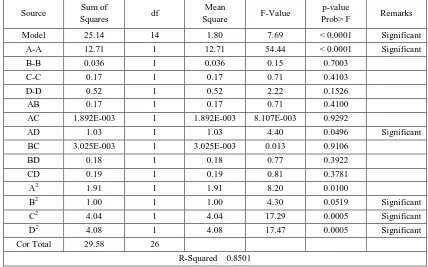
Table7. ANOVA Table for Kerf Width on machining of Al 7075-15%SiC
2) Regression Equation for Kerf Width: 93.59971-0.42297* Ton-2.21067* Toff-0.049942* Ip-0.077650* SV+3.75000E-003* Ton * Toff-3.00000E-005* Ton* Ip-5.40000E-004* Ton * SV-1.05000E-003* Toff * Ip-3.00000E-004* Toff * SV+5.45000E-004* Ip * SV+1.01833E-003* Ton2 +0.016958* Toff2+2.84583E-004* Ip2+1.63833E-003* SV2.
Source Sum of
Squares df
Mean
Square F-Value
p-value
Prob> F Remarks
Model 25.14 14 1.80 7.69 < 0.0001 Significant A-A 12.71 1 12.71 54.44 < 0.0001 Significant B-B 0.036 1 0.036 0.15 0.7003
C-C 0.17 1 0.17 0.71 0.4103
D-D 0.52 1 0.52 2.22 0.1526
AB 0.17 1 0.17 0.71 0.4100
AC 1.892E-003 1 1.892E-003 8.107E-003 0.9292
AD 1.03 1 1.03 4.40 0.0496 Significant BC 3.025E-003 1 3.025E-003 0.013 0.9106
BD 0.18 1 0.18 0.77 0.3922
CD 0.19 1 0.19 0.81 0.3781
A2 1.91 1 1.91 8.20 0.0100
B2 1.00 1 1.00 4.30 0.0519 Significant
C2 4.04 1 4.04 17.29 0.0005 Significant D2 4.08 1 4.08 17.47 0.0005 Significant Cor Total 29.58 26
[image:7.612.91.519.432.699.2]R-Squared 0.8501
3) Regression Equation for Surface Roughness: 1541.50563-1.91423*Ton-39.00900*Toff-2.57093*Ip-4.66618*SV-0.040700*Ton*Toff+4.35000E-004*Ton*SV+ 0.020260*Ton*SV-2.75000E-003*Toff*Ip+0.042300*Toff*SV-4.36000E-003*Ip*SV+0.019883*Ton2+0.3602*Toff2+7.22083E-003 *Ip2+0.029028*SV2
B. 3D Surface Plots for Process Responses Vs Process Variables
Fig3. Surface graph for interaction effect on Kerf Width for Al 7075-10% SiC
Fig4. Surface graph for interaction effect on Surface Roughness for Al 7075-10% SiC
Fig5. Surface graph for interaction effect on Kerf Width for Al 7075-15% SiC
Design-Expert® Sof tware Factor Coding: Actual KW (mm)
Design points abov e predicted v alue
Design points below predicted v alue
0.449
0.297
X1 = A: Ton X2 = B: Tof f
Actual Factors C: I p = 190 D: SV = 15
5 9 59 .5 60 60.5 6 1 100 1 02 10 4 10 6 108 110 0.25 0 .3 0 .35 0.4 0.4 5 K W ( m m )
A: Ton (micro sec) B: Toff (micro sec)
Design-Expert® Sof tware Factor C oding: Actual KW (m m )
D esign points abov e predicted v alue D esign points below predicted v alue
0.449
0.297 X1 = A: Ton X2 = C : Ip Actual Factors B: Tof f = 60 D: SV = 15
180 185 190 195 200 100 102 104 106 108 110 0.25 0.3 0.35 0.4 0.45 K W ( m m )
A: Ton (micro sec) C: Ip (Amp)
Design-Expert® Software Factor Coding: Actual SR (microns)
Design points above predicted value
Design points below predicted value
4.991
2.759
X1 = A: Ton X2 = B: Toff
Actual Factors C: Ip = 190 D: SV = 15
59 59.5 60 60.5 61 100 102 104 106 108 110 2.5 3 3.5 4 4.5 5 S R ( m ic ro n s )
A: Ton (micro sec) B: Toff (micro sec)
Design-Expert® Software Factor Coding: Actual SR (microns)
Design points above predicted value
Design points below predicted value
4.991
2.759
X1 = A: Ton X2 = C: Ip
Actual Factors B: Toff = 60 D: SV = 15
180 185 190 195 200 100 102 104 106 108 110 2.5 3 3.5 4 4.5 5 S R ( m ic ro n s )
A: Ton (micro sec) C: Ip (Amp)
Design-Expert® Software Factor Coding: Actual KW (mm)
Design points above predicted value
Design points below predicted value
0.397
0.303
X1 = A: Ton X2 = B: Toff
Actual Factors C: Ip = 190 D: SV = 15
59 59.5 60 60.5 61 100 102 104 106 108 110 0.28 0.3 0.32 0.34 0.36 0.38 0.4 K W ( m m )
A: Ton (micro sec) B: Toff (micro sec)
Design-Expert® Software Factor Coding: Actual KW (mm)
Design points above predicted value
Design points below predicted value
0.397
0.303
X1 = A: Ton X2 = C: Ip
Actual Factors B: Toff = 60 D: SV = 15
180 185 190 195 200 100 102 104 106 108 110 0.28 0.3 0.32 0.34 0.36 0.38 0.4 K W ( m m )
Fig6. Surface graph for interaction effect on Surface Roughness for Al 7075-15% SiC
IV.CONCLUSION
The important conclusions with the machining of Al 7075 -10% SiC and Al 7075 -15% SiC on Wire cut EDM using Response Surface Methodology includes as follows:
The optimal set of process parameters are identified for achieving minimum Surface Roughness and minimum Kerf width for each material.
Second order polynomial equation have been generated for both Surface Roughness and Kerf width.
ANOVA results to identify the effect of process parameters on process responses and percentage contribution of each parameter on process response
A. 7075-10% SiC
1) The optimal parameter setting for achieving minimum Kerf Width is obtained at 110μ sec of pulse on time and 60μ sec of pulse
off time 200 Amp of peak current and 15Volts of Spark gap voltage i.e 0.297 mm.
2) The optimal parameter setting for achieving minimum Surface Roughness is obtained at 110μ sec of pulse on time and 60 μ sec
of pulse off time 200 Amp of peak current and 15Volts of Spark gap voltage i.e 2.759 microns.
Al 7075-15% SiC
3) The optimal parameter setting for achieving minimum Kerf Width is obtained at 100 μ sec of pulse on time and 59 μ sec of
pulse off time 190 Amp of peak current and 15Volts of Spark gap voltage i.e 0.306mm
4) The optimal parameter setting for achieving minimum Surface Roughness is obtained at 100 μ sec of pulse on time and 60 μ sec
of pulse off time 200 Amp of peak current and 15 Volts of Spark gap voltage i.e 2.292 microns.
REFERENCES
[1] 1.Suresh Kumar.S, Uthayakumar.M, ThirumalaiKumaran.S, Parameswaran.P, Mohandas.E, Kempulraj.G, Ramesh Babu.B.S and Nataraan.S.A, 2015,‟
Parametric optimization of wire electrical discharge machining on aluminium alloy based composites through gray relational analysis” Journal of Manufacturing Process, Vol.20, PP.33-39.
[2] GanesdhDongre, SagarZawari, UdayDabade and SuhasJose.S, 2015, ‟Multi-objective optimization for Silicon wafer slicing usig Wire- EDM Process” Journa.l
of Material Science in Semiconductor processing, Vol.39, PP.793-806.
[3] AmiteshGoswami and Jatinder Kumar, 2014 ‟Investigation of surface integrity, material removal rate and wire wear ratio for WEDM of Nimonic 80A alloy using GRA and Taguchi method” Engineering Science and Technology, an International Journal, Vol.17 PP.173-184
[4] RavindranadhBobbili, Madhu.V and Gogia A.K., 2015‟ Multi response optimization of wire-EDM process parameters of ballistic grade aluminium alloy” Engineering Science and Technology, an International Journal, Vol.18, PP. 720-726.
[5] PujariSrinivasaRao, KoonaRamji and BeelaSathyanaranaya, 2014, ‟Experimental Investigation and optimization of Wire EDM For Surface Roughness MRR
and White layer in Machining of Aluminium alloy” International conference on advances in Manufacturing and Materials Engineering, AMME 2014, Vol.5,PP.2197-2206
Design-Expert® Software Factor Coding: Actual SR (microns)
Design points above predicted value
Design points below predicted value 6.79
3.027
X1 = A: Ton X2 = B: Ton
Actual Factors C: Ip = 190 D: SV = 15
59 59.5 60 60.5 61 100 102 104 106 108 110 2 3 4 5 6 7 S R ( m ic ro n s )
A: Ton (micro sec) B: Ton (micro sec)
Design-Expert® Software Factor Coding: Actual SR (microns)
Design points above predicted value
Design points below predicted value 6.79
3.027
X1 = A: Ton X2 = C: Ip
Actual Factors B: Ton = 60 D: SV = 15
180 185 190 195 200 100 102 104 106 108 110 2 3 4 5 6 7 S R ( m ic ro n s )
[6] AmrishRaj.D and Senthilvelan.T, 2015 ‟ Empirical Modelling and Optimization of Process Parameters of machining Titanium alloy by Wire-EDM using RSM” 4th International Conference on Materials Processing and Characterization,Vol.2, PP. 1682 – 1690