Quantifying Synergistic Information

(1)

In Partial Fulfillment of the Requirements

for the Degree of

Doctor of Philosophy

California Institute of Technology

Pasadena, California

2014

(2)

c 2014

Virgil Griffith

(3)

This thesis would not exist were it not for many people. Some of the prominent ones are Douglas

R. Hofstadter, for the inspiration; Giulio Tononi, for the theory; Christof Koch, for the ambition to

(4)

Acknowledgments

I wish to thank Christof Koch, Suzannah A. Fraker, Paul Williams, Mark Burgin, Tracey Ho, Edwin

(5)

Abstract

Within the microcosm of information theory, I explore what it means for a system to be functionally

irreducible. This is operationalized as quantifying the extent to which cooperative or “synergistic”

e↵ects enable random variables X1, . . . , Xn to predict (have mutual information about) a single

target random variableY. In Chapter 1, we introduce the problem with some emblematic examples.

In Chapter 2, we show how six di↵erent measures from the existing literature fail to quantify this

notion of synergistic mutual information. In Chapter 3, we take a step towards a measure of synergy

which yields the first nontrivial lowerbound on synergistic mutual information. In Chapter 4, we

find that synergy is but the weakest notion of a broader concept ofirreducibility. In Chapter 5, we apply our results from Chapters 3 and 4 towards grounding Giulio Tononi’s ambitious measure,

(6)

What is Synergy?

The prior literature [24, 30, 1, 6, 19, 36] has termed several distinct concepts as “synergy”. We

define synergy as a special case of irreducibility—specifically, synergy is irreducibility to atomic elements. By definition, a group of two or more agents synergistically perform a task if and only if

the performance of that task decreases when the agents work “separately”, or in parallel isolation.

It is important to remember that it is the collective action that is irreducible, not the agents themselves. A concrete example of irreducibility is the “agents” hydrogen and oxygen working to

extinguish fire. Even when H2and O2are both present in the same container, if working separately

neither extinguishes fire (on the contrary, fire grows!). But hydrogen and oxygen fused or “grouped”

into a single entity, H2O, readily extinguishes fire.

The concept of synergy spans many fields and theoretically could be applied to any non-subadditive

function. But within the confines of Shannon information theory, synergy—or more formally, syner-gistic information—is a property of a set ofnrandom variablesX={X1, X2, . . . , Xn} cooperating to predict, that is, reduce the uncertainty of, a single target random variableY.

1.1 Notation and PI-diagrams

We use the following notation throughout. Let

n: The number of predictorsX1, X2, . . . , Xn. n 2.

X1...n: The joint random variable (cartesian product) of allnpredictorsX1X2. . . Xn.

Xi: Thei’th predictor random variable (r.v.). 1in.

X: Theset of allnpredictors{X1, X2, . . . , Xn}.

Y: Thetarget r.v. to be predicted.

(11)

1.1.1 Understanding PI-diagrams

Partial information diagrams (PI-diagrams), introduced by [36], extend Venn diagrams to properly

represent synergy. Their framework has been invaluable to the evolution of our thinking on synergy.

A PI-diagram is composed of nonnegative partial information regions (PI-regions). Unlike the standard Venn entropy diagram in which the sum of all regions is the joint entropy H(X1...n, Y),

in PI-diagrams the sum of all regions (i.e. the space of the PI-diagram) is the mutual

informa-tion I(X1...n:Y). PI-diagrams are immensely helpful in understanding how the mutual information

I(X1...n:Y) is distributed across the coalitions and singletons ofX.1

{12}

{1}

{2}

{1,2}

(a)n= 2

{1} {2}

{3}

{12}

{13} {23}

{1,2}

{1,3} {2,3}

{1,2,3}

{12,13} {12,23}

{12,13,23}

{2,13} {1,23}

{3,12} {123}

{13,23}

*

* *

[image:11.612.126.515.316.573.2]

(b)n= 3

Figure 1.1: PI-diagrams for two and three predictors. Each PI-region represents nonnegative in-formation about Y. A PI-region’s color represents whether its information is redundant (yellow), unique (magenta), or synergistic (cyan). To preserve symmetry, the PI-region “_{12,13,23_}” is dis-played as three separate regions each marked with a “*”. All three *-regions should be treated as though they are a single region.

How to read PI-diagrams. Each PI-region is uniquely identified by its “set notation” where

each element is denoted solely by the predictors’ indices. For example, in the PI-diagram forn= 2

1_{Formally, how the mutual information is distributed across the set of all nonempty antichains on the powerset of}

(12)

(Figure 1.1a): _{1_} is the information about Y only X1 carries (likewise {2} is the information

only X2 carries); {1,2} is the information about Y that X1 as well as X2 carries, while {12} is

the information aboutY that is specified only by the coalition (joint random variable)X1X2. For

getting used to this way of thinking, common informational quantities are represented by colored

regions in Figure 5.5.

{12}

{1} {2}

{1,2}

(a) I(X1:Y)

{12}

{1} {2}

{1,2}

(b) I(X2:Y)

{12}

{1} {2}

{1,2}

(c) I X1:Y|X2

{12}

{1} {2}

{1,2}

(d) I X2:Y|X1

{12}

{1} {2}

{1,2}

(e) I(X1X2:Y)

Figure 1.2: PI-diagrams forn= 2 representing standard informational quantities.

The general structure of a PI-diagram becomes clearer after examining the PI-diagram forn= 3

(Figure 1.1b). All PI-regions fromn= 2 are again present. Each predictor (X1, X2, X3) can carry

unique information (regions labeled _{1_}, _{2_}, _{3_}), carry information redundantly with another

predictor (_{1,2_}, _{1,3_}, _{2,3_}), or specify information through a coalition with another predictor

(_{12_}, _{13_}, _{23_}). New in n = 3 is information carried by all three predictors (_{1,2,3_}) as well

as information specified through a three-way coalition (_{123_}). Intriguingly, for three predictors,

information can be provided by a coalition as well as a singleton (_{1,23_},_{2,13_},_{3,12_}) or specified

by multiple coalitions ({12,13},{12,23},{13,23},{12,13,23}).

1.2 Information can be redundant, unique, or synergistic

Each PI-region represents an irreducible nonnegative slice of the mutual information I(X1...n:Y)

that is either:

1. Redundant. Information carried by a singleton predictor as well as available somewhere else.

Forn= 2: _{1,2_}. Forn= 3: _{1,2_},_{1,3_},_{2,3_},_{1,2,3_},_{1,23_},_{2,13_},_{3,12_}.

2. Unique. Information carried by exactly one singleton predictor and available nowhere else.

Forn= 2: {1},{2}. Forn= 3: {1}, {2},{3}.

3. Synergistic. Any and all information in I(X1...n:Y) that is not carried by a singleton

predic-tor. n= 2: {12}. Forn= 3: {12},{13},{23},{123},{12,13},{12,23},{13,23},{12,13,23}.

Although a single PI-region is either redundant, unique, or synergistic, a single state of the

target can have any combination of positive PI-regions, i.e. a single state of the target can convey

(13)

ExaminingX1orX2 identically specifies one bit ofY, thus we say setX={X1, X2}has one bit of

redundant information aboutY.

X1 X2 Y

r r r 1_/₂

R R R 1_/₂

(a) Pr(x1, x2, y)

½ r

½ R

(b) circuit diagram

0 0

0 +1 {12}

{1} {2}

{1,2}

(c) PI-diagram

Figure 1.3: Example Rdn. Figure 1.3a shows the joint distribution of r.v.’s X1, X2, and Y, and

the joint probability Pr(x1, x2, y) is along the right-hand side of (a), revealing that all three terms

are fully correlated. Figure 1.3b represents the joint distribution as an electrical circuit. Fig-ure 1.3c is the PI-diagram indicating that set _{X1, X2} has 1 bit of redundant information about

Y. I(X1X2:Y) = I(X1:Y) = I(X2:Y) = H(Y) = 1 bit.

1.2.2 Example Unq: Unique information

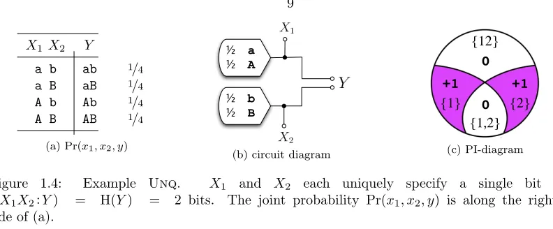
PredictorXicarriesunique informationaboutY if and only ifXispecifies information aboutY that is not specified by anything else (a singleton or coalition of the othern 1 predictors). Figure 1.4

illustrates a simple case of unique information. Y has four equiprobable states: ab, aB, Ab, and AB.X1 uniquely specifies bita/A, andX2 uniquely specifies bitb/B. If we had instead labeled the

Y-states: 0,1,2, and3,X1andX2would still have strictly unique information aboutY. The state

ofX1would specify between{0,1}and{2,3}, and the state ofX2would specify between{0,2}and

{1,3}—together fully specifying the state ofY.

1.2.3 Example Xor: Synergistic information

A set of predictorsX={X1, . . . , Xn}has synergistic information about Y if and only if the whole

(X1...n) specifies information aboutY that is not specified by any singleton predictor. The canonical

example of synergistic information is theXor-gate (Figure 1.5). In this example, the wholeX1X2

fully specifiesY,

I(X1X2:Y) = H(Y) = 1 bit,

2_X₁_and_X₂_{providing identical information about}_Y _{is di}_↵_{erent from providing the same}_magnitude_{of information} aboutY, i.e. I(X1:Y) = I(X2:Y). ExampleUnq(Figure 1.4) is an example where I(X1:Y) = I(X2:Y) = 1 bit yet

(14)

X1X2 Y

a b ab 1_/₄

a B aB 1_/₄

A b Ab 1_/₄

A B AB 1_/₄

(a) Pr(x1, x2, y)

½ a

½ A

½ b

½ B

(b) circuit diagram

+1 0 +1 0 {12} {1} {2} {1,2} (c) PI-diagram

Figure 1.4: Example Unq. X1 and X2 each uniquely specify a single bit of Y.

I(X1X2:Y) = H(Y) = 2 bits. The joint probability Pr(x1, x2, y) is along the right-hand

side of (a).

but the singletonsX1andX2specify nothing aboutY,

I(X1:Y) = I(X2:Y) = 0 bits.

With bothX1andX2themselves having zero information aboutY, we know that there can not be

any redundant or unique information aboutY, that the three PI-regions_{1_} = _{2_} = _{1,2_} = 0

bits. As the information between X1X2 and Y must come from somewhere, by elimination we

conclude thatX1 andX2 synergistically specifyY.

X1X2 Y

0 0 0 1_/₄

0 1 1 1_/₄

1 0 1 1_/₄

1 1 0 1_/₄

(a) Pr(x1, x2, y)

½ 0

½ 1

½ 0

½ 1 X1

X2

Y XOR

(b) circuit diagram

[image:14.612.116.512.57.221.2]

0 +1 0 0 {12} {1} {2} {1,2} (c) PI-diagram

Figure 1.5: Example Xor. X1 andX2 synergistically specify Y. I(X1X2:Y) = H(Y) = 1 bit.

(15)

Chapter 2

Six Prior Measures of Synergy

2.1 Definitions

2.1.1 Multivariate Mutual Information:

MMI(

X

1

;

· · ·

;

X

n

;

Y

)

The first information-theoretic measure of synergy dates to 1954 from [24]. Inspired by Venn

en-tropy diagrams, they defined themultivariate mutual information (MMI), MMI(X1;· · ·;Xn;Y)⌘

P

T✓{X1,...,Xn,Y}( 1)

|T|+1_H(_T_{). Negative MMI was understood to be synergy. Therefore the MMI}

measure of synergy is,

SMMI(X1;· · ·;Xn;Y)⌘

X

T✓{X1,...,Xn,Y}

( 1)|T|+1H(T)

= X

T✓{X1,...,Xn,Y}

( 1)|T|H(T) .

(2.1)

2.1.2 Interaction Information:

_II

(

X

1

;

· · ·

;

X

n

;

Y

)

Interaction information (_II), sometimes called the co-information, was introduced in [6] and tweaks

MMI synergy measure. Although intended to measure informational “groupness” [6], Interaction

Information is commonly interpreted as the magnitude of “information bound up in a set of variables,

beyond that which is present in any subset of those variables.”1

Interaction Information among thenpredictors andY is defined as,

II(X1;· · · ;Xn;Y)⌘( 1)nSMMI(X1;· · ·;Xn;Y)

= X

T✓{X1,...,Xn,Y}

( 1)n |T|H(T) . (2.2)

(16)

Interaction Information is a signed measure where a positive value signifies synergy and a negative

value signifies redundancy. Representing Interaction Information as a PI-diagram (Figure 2.1) reveals

an intimidating imbroglio of added and subtracted PI-regions.

{12}

{1}

{2}

{1,2}

(a)II({X1, X2}:Y)

{1} {2} {3} {12} {13} {23} {1,2} {1,3} {2,3} {1,2,3} {12,13} {12,23} {12,13,23} {2,13} {1,23} {3,12} {123} {13,23} * * *

[image:16.612.192.453.146.330.2]

(b)II(X1;X2;X3;Y)

Figure 2.1: PI-diagrams illustrating interaction information forn= 2 (left) and n= 3 (right). The colors denote the added and subtracted PI-regions. WMS (X:Y) is the green PI-region(s), minus the orange PI-region(s), minus two times any red PI-region.

2.1.3 WholeMinusSum synergy:

WMS (

X

:

Y

)

The earliest known sightings of bivariate WholeMinusSum synergy (WMS) are in [13, 12], with the

general case in [11]. WholeMinusSum synergy is a signed measure where a positive value signifies

synergy and a negative value signifies redundancy. WholeMinusSum synergy is defined by eq. (2.3)

and interestingly reduces to eq. (2.5)—the di↵erence of twototal correlations.2

WMS (X:Y) _⌘ I(X1...n:Y) n

X

i=1

I(Xi:Y) (2.3)

= n

X

i=1

H Xi|Y H X1...n|Y

2 4

n

X

i=1

H(Xi) H(X1...n)

3

5 (2.4)

= TC (X1;· · ·;Xn|Y) TC (X1;· · · ;Xn) (2.5)

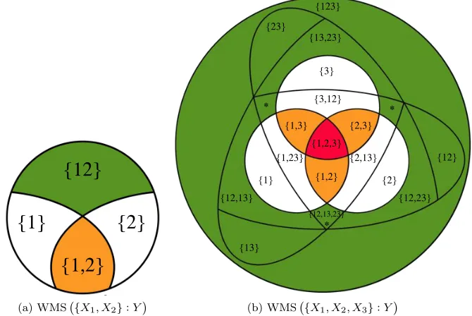
Representing eq. (2.3) for n= 2 as a PI-diagram (Figure 2.2a) reveals that WMS is the synergy

betweenX1 and X2 minus their redundancy. Thus, when there is an equal magnitude of synergy

and redundancy betweenX1 andX2, WholeMinusSum synergy iszero—leading one toerroneously

2_TC(_X

(17)

{12}

{1}

{2}

{1,2}

(a) WMS {X1, X2}:Y

{1} {2}

{3}

{12}

{13} {23}

{1,2} {1,3} {2,3}

{1,2,3}

{12,13} {12,23}

{12,13,23} {2,13} {1,23}

{3,12} {123}

{13,23}

*

* *

(b) WMS {X1, X2, X3}:Y

Figure 2.2: PI-diagrams illustrating WholeMinusSum synergy for n = 2 (left) and n = 3 (right). The colors denote the added and subtracted PI-regions. WMS (X:Y) is the green PI-region(s) minus the orange PI-region(s) minus two times any red PI-region.

2.1.4 WholeMinusPartitionSum:

WMPS (

X

:

Y

)

WholeMinusPartitionSum, denoted WMPS (X:Y), is a stricter generalization of WMS synergy for

n >2. It was introduced in [34, 1] and is defined as,

WMPS (X:Y)⌘I(X1...n:Y) max

P

|P|

X

i=1

I(Pi:Y) , (2.6)

where Penumerates over all partitions of the set of predictors {X1, . . . , Xn}.

WholeMinusPar-titionSum is a signed measure where a positive value signifies synergy and a negative value signifies

redundancy.

For n = 3, there are four partitions of X resulting in four possible PI-diagrams—one for each

partition. Figure 2.3 depicts the four possible values of WMPS(_{X1, X2, X3} : Y). Because

{X1, . . . , Xn} is a possible partition ofX, WMPS(X:Y)WMS(X:Y).

[image:17.612.154.489.167.391.2]

(18)

{12}

{1}

{2}

{1,2}

(a) WMPS {X1, X2}:Y

{1} {2} {3} {12} {13} {23} {1,2} {1,3} {2,3} {1,2,3} {12,13} {12,23} {12,13,23} {2,13} {1,23} {3,12} {123} {13,23} * * *

(b)P={X1, X2, X3}

{1} {2} {3} {12} {13} {23} {1,2} {1,3} {2,3} {1,2,3} {12,13} {12,23} {12,13,23} {2,13} {1,23} {3,12} {123} {13,23} * * *

(c)P={X1X2, X3}

{1} {2} {3} {12} {13} {23} {1,2} {1,3} {2,3} {1,2,3} {12,13} {12,23} {12,13,23} {2,13} {1,23} {3,12} {123} {13,23} * * *

(d)P={X1X3, X2}

{1} {2} {3} {12} {13} {23} {1,2} {1,3} {2,3} {1,2,3} {12,13} {12,23} {12,13,23} {2,13} {1,23} {3,12} {123} {13,23} * * *

[image:18.612.159.491.200.580.2]

(e)P={X2X3, X1}

Figure 2.3: PI-diagrams depicting WholeMinusPartitionSum synergy for n= 2 (2.3a) and n = 3 (2.3b–2.3e). Each measure is the green PI-regions minus the orange PI-regions minus two times any red PI-region. WMPS _{X1, X2, X3}:Y is theminimum value over subfigures 2.3b–2.3e.

2.1.5 I

max

synergy:

S

max

(

X

:

Y

)

Imaxsynergy, denotedSmax, was the first synergy measure derived from Partial Information Decomposition[36].

(19)

where I(Xi:Y =y) is [10]’s “specific-surprise”,

I(Xi:Y =y) ⌘ DKL

h

Pr Xi|y Pr(Xi)

i

(2.9)

= X

xi2Xi

Pr xi|y log

Pr(xi, y)

Pr(xi) Pr(y) . (2.10)

There are two major advantages of_Smaxsynergy. Smaxis not only nonnegative, but also invariant

to duplicate predictors.

2.1.6 Correlational importance:

I (

X

;

Y

)

Correlational importance, denoted I, comes from [27, 25, 26, 28, 21]. Correlational importance

quantifies the “informational importance of conditional dependence” or the “information lost when

ignoring conditional dependence” among the predictors decoding target Y. On casual inspection,

I seems related to our intuitive conception of synergy. I is defined as,

I (X;Y) ⌘ DKL

h

Pr Y|X1...n Prind(Y|X)

i

(2.11)

= X

y,x2Y,X

Pr(y, x1...n) log

Pr y_|x1...n Prind(y|x)

, (2.12)

where Prind y|x ⌘

Pr(y)Qn

i=1Pr(xi|y)

P

y0Pr(y0)Qni=1Pr(xi|y0). After some algebra

4_{eq. (2.12) becomes,}

I (X;Y) = TC (X1;· · ·;Xn|Y) DKL

2

4Pr(X1...n)

X

y Pr(y)

n

Y

i=1

Pr Xi|y

3

5 . (2.13)

I is conceptually innovative, yet examples reveal that I measures something ever-so-subtly

di↵erent from intuitive synergistic information.

(20)

2.2 The six prior measures are not equivalent

For n= 2, the four measures _SMMI, II, WMS, and WMPS are equivalent. But in general, none

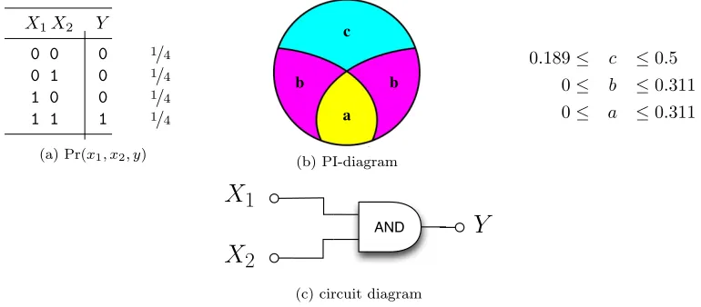
of these six measures are equivalent. ExampleAnd (Figure 2.4) shows that_Smax and I are not

equivalent. Example XorMultiCoal(Figure 2.5) shows that _SMMI, II, WMS, and WMPS are

not equivalent.

X1X2 Y

0 0 0 1_/₄

0 1 0 1_/₄

1 0 0 1_/₄

1 1 1 1_/₄

(a) Pr(x1, x2, y)

c

b

a b

(b) PI-diagram

0.189 c 0.5 0_ b _0.311 0 a 0.311

Y

X

₁

X

₂

AND

[image:20.612.127.512.189.358.2]

(c) circuit diagram

Figure 2.4: ExampleAnd. The exact PI-decomposition of an AND-gate remains uncertain. But we can bounda, b, andc using WMS and_Smax.

Example SMMI II WMS WMPS Smax I

And 0.189 0.189 0.189 0.189 1_/₂ _0.104

XorMultiCoal 2 –2 1 0 1 1

Table 2.1: Examples demonstrating that the six prior measures are not equivalent.

2.3 Counter-intuitive behaviors of the six prior measures

2.3.1 I

max

synergy:

S

max

Despite several desired properties, _Smax sometimes miscategorizes merely unique information as

synergistic. This can be seen in exampleUnq(Figure 1.4). In exampleUnq, the wires in Figure 1.4b

don’t even touch, yet Smax asserts there is one bit of synergy and one bit of redundancy—this is

palpably strange.

A more abstract way to understand whySmaxoverestimates synergy is to imagine a hypothetical

example where there are exactly two bits of unique information for every state y ₂ Y and no

(21)

Ab Ac bc 1 1_/₈

aB ac Bc 1 1_/₈

ab aC bC 1 1_/₈

AB AC BC 1 1_/₈

(a) Pr(x1, x2, x3, y)

X

₃

c/C

(b) circuit diagram

+1

{1} {2}

{3}

{12}

{13} {23}

{1,2}

{1,3} {2,3}

{1,2,3}

{12,13} {12,23}

{12,13,23} {2,13} {1,23}

{3,12} {123}

{13,23}

*

* *

[image:21.612.141.521.66.409.2]

(c) PI-diagram

Figure 2.5: Example XorMultiCoaldemonstrates how the same information can be specified by multiple coalitions. In XorMultiCoal the target Y has one bit of uncertainty, H(Y) = 1 bit, and Y is the parity of three incoming wires. Just as the output of Xor is specified only after knowing the state of both inputs, the output of XorMultiCoal is specified only after knowing the state of all three wires. Each predictor is distinct and has access to two of the three incom-ing wires. For example, predictor X1 has access to the a/A and b/Bwires, X2 has access to the

a/A and c/C wires, and X3 has access to the b/B and c/C wires. Although no single predictor

specifies Y, any coalition of two predictors has access to all three wires and fully specifies Y, I(X1X2:Y) = I(X1X3:Y) = I(X2X3:Y) = H(Y) = 1 bit. In the PI-diagram this puts

one bit in PI-region{12,13,23} and zero everywhere else.

predictors, which would be the max [1,1] = 1 bit. TheSmax synergy would then be 2 1 = 1 bit of

synergy, even though by definition there was no synergy, but merely two bits of unique information.

Altogether, we conclude thatSmaxoverestimatesthe intuitive synergy by miscategorizing merely

unique information as synergistic whenever two or more predictors have unique information about

the target.

2.3.2 S

MMI

,

II

,

WMS

,

WMPS

All four of these measures are equivalent for n = 2. Given this agreement, it is ironic that there

(22)

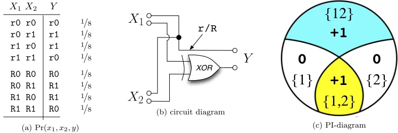
redundancy” behavior forn= 2 is exampleRdnXor(Figure 2.6), which overlays examplesRdnand

Xor to form a single system. The targetY has two bits of uncertainty, i.e. H(Y) = 2. LikeRdn,

eitherX1 orX2identically specifies the letter ofY (r/R), making one bit of redundant information.

Like Xor, only the coalition X1X2 specifies the digit of Y (0/1), making one bit of synergistic

information. Together this makes one bit of redundancy and one bit of synergy. We assert that for

n= 2, all four measuresunderestimatethe synergy. Equivalently, we say that their answer forn= 2 is alowerbound on the intuitive synergy.

Note that in RdnXorevery state y2Y conveys one bit of redundant information and one bit

of synergistic information, e.g. for the statey =r0the letter “r” is specified redundantly and the digit “0” is specified synergistically.

X1X2 Y

r0 r0 r0 1_/₈

r0 r1 r1 1_/₈

r1 r0 r1 1_/₈

r1 r1 r0 1_/₈

R0 R0 R0 1_/₈

R0 R1 R1 1_/₈

R1 R0 R1 1_/₈

R1 R1 R0 1_/₈

(a) Pr(x1, x2, y)

X

₂

XOR

Y

X

₁

r/R

(b) circuit diagram

0 +1

{12}

{1}

{2}

[image:22.612.120.528.262.399.2]

{1,2}

(c) PI-diagram

Figure 2.6: Example RdnXor has one bit of redundancy and one bit of synergy. Yet for this example, the four most common measures of synergy arrive at zero bits.

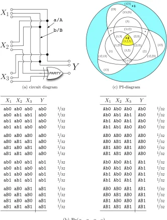
Our next example, ParityRdnRdn(Figure 2.7), has one bit of synergy and two bits of

redun-dancy for a total of I(X1X2X3:Y) = H(Y) = 3 bits. It emphasizes the disagreement between II

and measures SMMI, WMS, and WMPS. If SMMI, WMS, or WMPS were always simply “synergy

minus redundancy”, then one of them would calculate 1 2 = 1 bits. But for this example all

three measures subtracts redundanciesmultiple times to calculate 1 (2_·2) = 3 bits, signifying all three bits of H(Y) are specified redundantly. _II makes a di↵erent misstep. Instead of subtracting

redundancy multiple times, for n= 3 _II adds the maximum redundancy to calculate 1 + 2 = +3 bits, signifying three bits of synergy and no redundancy. Both answers are palpably mistaken.

2.3.3 Correlational importance:

I

The first concerning example is [29]’s Figure 4, where I exceeds the mutual information I(X1...n:Y)

with I (X;Y) = 0.0145 and I(X1...n:Y) = 0.0140. This fact alone prevents interpreting I

the magnitude of mutual I(X1...n:Y) arising from correlational dependence.

Could I upperbound synergy instead? We turn to example And (Figure 2.4) with n = 2

(23)

Taking both together, we conclude that I measures something fundamentally di↵erent from

synergistic information.

Example _SMMI II WMS WMPS Smax I

Unq 0 0 0 0 1 0

RdnXor 0 0 0 0 1 1

ParityRdnRdn –3 3 –3 –3 1 1

And 0.189 0.189 0.189 0.189 1_/₂ _0.104

(24)

X

₂

PARITY

Y

X

₁

X

₃

a/A b/B

(a) circuit diagram

+2 +1 {1} {2} {3} {12} {13} {23} {1,2} {1,3} {2,3} {1,2,3} {12,13} {12,23} {12,13,23} {2,13} {1,23} {3,12} {123} {13,23} * * * (c) PI-diagram

X1 X2 X3 Y

ab0 ab0 ab0 ab0 1_/₃₂

ab0 ab1 ab1 ab0 1_/₃₂

ab1 ab0 ab1 ab0 1_/₃₂

ab1 ab1 ab0 ab0 1_/₃₂

aB0 aB0 aB0 aB0 1_/₃₂

aB0 aB1 aB1 aB0 1_/₃₂

aB1 aB0 aB1 aB0 1_/₃₂

aB1 aB1 aB0 aB0 1_/₃₂

ab0 ab0 ab1 ab1 1_/₃₂

ab0 ab1 ab0 ab1 1_/₃₂

ab1 ab0 ab0 ab1 1_/₃₂

ab1 ab1 ab1 ab1 1_/₃₂

aB0 aB0 aB1 aB1 1_/₃₂

aB0 aB1 aB0 aB1 1_/₃₂

aB1 aB0 aB0 aB1 1_/₃₂

aB1 aB1 aB1 aB1 1_/₃₂

X1 X2 X3 Y

Ab0 Ab0 Ab0 Ab0 1_/₃₂

Ab0 Ab1 Ab1 Ab0 1_/₃₂

Ab1 Ab0 Ab1 Ab0 1_/₃₂

Ab1 Ab1 Ab0 Ab0 1_/₃₂

AB0 AB0 AB0 AB0 1_/₃₂

AB0 AB1 AB1 AB0 1_/₃₂

AB1 AB0 AB1 AB0 1_/₃₂

AB1 AB1 AB0 AB0 1_/₃₂

Ab0 Ab0 Ab1 Ab1 1_/₃₂

Ab0 Ab1 Ab0 Ab1 1_/₃₂

Ab1 Ab0 Ab0 Ab1 1_/₃₂

Ab1 Ab1 Ab1 Ab1 1_/₃₂

AB0 AB0 AB1 AB1 1_/₃₂

AB0 AB1 AB0 AB1 1_/₃₂

AB1 AB0 AB0 AB1 1_/₃₂

AB1 AB1 AB1 AB1 1_/₃₂

[image:24.612.157.489.151.588.2]

(b) Pr(x1, x2, x3, y)

Figure 2.7: Example ParityRdnRdn. Three predictors redundantly specify two bits of Y, I(X1:Y) = I(X2:Y) = I(X3:Y) = 2 bits. At the same time, the three predictors holistically

(25)

Appendix

2.A

Algebraic simplification of

I

Prior literature [25, 26, 28, 21] defines I (X;Y) as,

I (X;Y) _⌘ DKL

h

Pr Y_|X1...n Prind(Y|X)

i

(2.14)

= X

x,y2X,Y

Pr(x, y) log Pr y|x

Prind(y|x) . (2.15)

Where,

Prind(Y =y|X=x) ⌘

Pr(y) Prind(X=x|Y =y)

Prind(X=x) (2.16)

= Pr(y)

Qn

i=1Pr xi|y Prind(x)

(2.17)

Prind(X=x) ⌘

X

y2Y

Pr(Y =y) n

Y

i=1

Pr xi|y (2.18)

(26)

I (X;Y) = X

x,y2X,Y

Pr(x, y) log Pr y|x Prind(y|x)

(2.19)

= X

x,y2X,Y

Pr(x, y) log Pr y|x Prind(x) Pr(y)Qn_i₌₁Pr xi|y

(2.20)

= X

x,y2X,Y

Pr(x, y) log_QnPr x|y i=1Pr xi|y

Prind(x)

Pr(x) (2.21)

= X

x,y2X,Y

+ X

x,y2X,Y

Pr(x, y) logPrind(x) Pr(x)

= X

x,y2X,Y

X

x2X

Pr(x) log Pr(x) Prind(x)

(2.22)

= DKL

2

4Pr X1...n|Y n

Y

i=1

Pr Xi|Y

3

5 DKL⇥Pr(X1...n) Prind(X)⇤

= TC (X1;· · · ;Xn|Y) DKL⇥Pr(X1...n) Prind(X)⇤ . (2.23)

(27)

Part II

(28)

Chapter 3

First Nontrivial Lowerbound on

Synergy

Remark: This chapter borrows liberally from the joint paper [14].

3.1 Introduction

Introduced in [36],Partial Information Decomposition (PID) is an immensely useful framework for deepening our understanding of multivariate interactions, particularly our understanding of

infor-mational redundancy and synergy. To harness the PID framework, the user brings her own measure

ofintersection information, I\(X1, . . . , Xn:Y), which quantifies the magnitude of information that each of thenpredictorsX1, . . . , Xn conveys “redundantly” about a target random variable Y. An

antichain lattice of redundant, unique, and synergistic partial informations is built from the

inter-section information.

In [36], the authors propose to use the following quantity, Imin, as the intersection information

measure:

Imin(X1, . . . , Xn :Y)⌘

X

y

Pr(y) min

i I(Xi:Y =y)

=X

y

Pr(y) min i DKL

h

Pr Xi|y Pr(Xi)

i

,

(3.1)

where DKLis the Kullback-Leibler divergence.

Though Iminis an intuitive and plausible choice for the intersection information, [15] showed that

Imin has counterintuitive properties. In particular, Imincalculates one bit of redundant information

for exampleunq(Figure 3.3). It does this because each input shares one bit of information with the

output. However, it is quite clear that the shared informations are, in fact, di↵erent: X1 provides

the low bit, while X2 provides the high bit. This led to the conclusion that Imin over-estimates

(29)

Here we do not definitively solve this problem, but we present a strong candidate intersection

information measure for the special case ofzero-errorinformation. This is useful in of itself because it provides a template for how the yet undiscovered ideal intersection information measure for Shannon

mutual information could work. Alternatively, if a Shannon intersection information measure with

the same properties does not exist, then we have learned something significant.

In the next section, we introduce some definitions, some notation, and a necessary lemma. We also

extend and clarify the desired properties for intersection information. In Section 3.4 we introduce

zero-error information and its intersection information measure. In Section 3.5 we use the same

methodology to produce a novel candidate for the Shannon intersection information. In Section 3.6

we show the successes and shortcomings of our candidate intersection information measure using

example circuits. Finally, in Section 3.8 we summarize our progress towards the ideal intersection

information measure and suggest directions for improvement. The Appendix is devoted to technical

lemmas and their proofs, to which we refer in the main text.

3.2 Two examples elucidating desired properties for synergy

To help the reader develop intuition for any proper measure of synergy, we illustrate some desired

properties of synergistic information with pedagogical examples. Both examples are derived from

exampleXor.

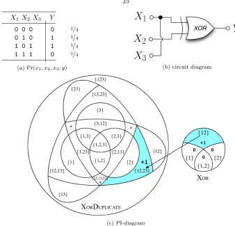
3.2.1 XorDuplicate: Synergy is invariant to duplicating a predictor

ExampleXorDuplicate (Figure 3.1) adds a third predictor,X3, a copy of predictorX1, toXor.

Whereas inXor the target Y is specified only by coalition X1X2, duplicating predictor X1 as X3

makes the target equally specifiable by coalitionX3X2.

Although now two di↵erent coalitions identically specify Y, mutual information is invariant to

duplicates, e.g. I(X1X2X3:Y) = I(X1X2:Y) bit. For synergistic information to be likewise bounded

between zero and the total mutual information I(X1...n:Y), synergistic information must similarly

be invariant to duplicates, e.g. the synergistic information between set _{X1, X2} and Y must be

the same as the synergistic information between _{X1, X2, X3}and Y. This makes sense because if

synergistic information is defined as the information in the whole beyond its parts, duplicating a part

(30)

X1X2 X3 Y

0 0 0 0 1_/₄

0 1 0 1 1_/₄

1 0 1 1 1_/₄

1 1 1 0 1_/₄

(a) Pr(x1, x2, x3, y)

Y

X

₁

X

₂

X

₃

XOR

(b) circuit diagram

+1 {1} {2} {3} {12} {13} {23} {1,2} {1,3} {2,3} {1,2,3} {12,13} {12,23} {12,13,23} {2,13} {1,23} {3,12} {123} {13,23} * * * 0 +1 0 0 {12} {1} {2} {1,2}

XORDUPLICATE

XOR

[image:30.612.143.481.58.383.2]

(c) PI-diagram

Figure 3.1: ExampleXorDuplicate shows that duplicating predictorX1 as X3 turns the

single-coalition synergy_{12_}into the multi-coalition synergy_{12,23_}. After duplicatingX1, the coalition

X3X2 as well as coalition X1X2 specifies Y. Synergistic information is unchanged from Xor,

I(X3X2:Y) = I(X1X2:Y) = H(Y) = 1 bit.

3.2.2 XorLoses: Adding a new predictor can decrease synergy

ExampleXorLoses(Figure 3.2) adds a third predictor,X3, toXorand concretizes the distinction

between synergy and “redundant synergy”. InXorLoses the targetY has one bit of uncertainty,

and just as in example Xorthe coalition X1X2 fully specifies the target, I(X1X2:Y) = H(Y) = 1

bit. However, XorLoseshas zero intuitive synergy because the newly added singleton predictor,

X3, fully specifiesY by itself. This makes the synergy betweenX1 andX2 completely redundant—

everything the coalitionX1X2 specifies is now already specified by the singletonX3.

3.3 Preliminaries

3.3.1 Informational Partial Order and Equivalence

We assume an underlying probability space on which we define random variables, as denoted by

(31)

1 1 0 0 1_/₄

(a) Pr(x1, x2, x3, y)

Y

XOR

(b) circuit diagram

+1

0 +1

0 0

{12}

{1} {2}

{1,2}

XOR

XORLOSES

{1} {2}

{3}

{12}

{13} {23}

{1,2} {1,3} {2,3}

{1,2,3}

{12,13} {12,23}

{12,13,23}

{2,13} {1,23}

{3,12} {123}

{13,23}

*

* *

[image:31.612.149.480.71.426.2]

(c) PI-diagram

Figure 3.2: Example XorLoses. Target Y is fully specified by the coalition X1X2 as well as by

the singleton X3. I(X1X2:Y) = I(X3:Y) = H(Y) = 1 bit. Therefore, the information

synergistically specified by coalitionX1X2 is a redundant synergy.

on finite spaces.

Given random variables X and Y, we write X Y to signify that there exists a measurable

functionf such that X =f(Y). In this case, following the terminology in [22], we say that X is

informationally poorerthanY; this induces a partial order on the set of random variables. Similarly, we writeX ⌫Y ifY X, in which case we sayX isinformationally richer thanY.

IfX andY are such thatX Y andX_⌫Y, then we writeX ⇠=Y. In this case, again following

[22], we say that X and Y are informationally equivalent. In other words, X ⇠=Y if and only if there’s an invertible function between X and Y, i.e., one can relabel the values of X to obtain a

random value that is equal toY and vice versa.

This “information-equivalence” relation can easily be shown to be an equivalence relation, so that

we can partition the set of all random variables into disjoint equivalence classes. The ordering is

invariant within these equivalence classes in the following sense: ifX Y andY ⇠=Z, thenX Z.

(32)

is invariant, as stated formally in Lemma 3.3.1 below.

3.3.2 Information Lattice

Next, we follow [22] and consider the join and meet operators. These operators were defined for

information elements, which are -algebras, or, equivalently, equivalence classes of random variables. We deviate from [22], though, by defining the join and meet operators for random variables, but we

do preserve their conceptual properties.

Given random variables X and Y, we define X gY (called the join of X and Y) to be an informationally poorest (“smallest” in the sense of the partial order ) random variable such that

X XgY andY XgY. In other words, ifZ is such thatX Z andY Z, thenXgY Z. Note thatXgY is unique only up to equivalence with respect to⇠=. In other words,XgY does not define a specific, unique random variable. Nonetheless, standard information-theoretic quantities

are invariant over the set of random variables satisfying the condition specified above. For example,

the entropy ofXgY is invariant over the entire equivalence class of random variables satisfying the condition above (by Lemma 3.3.1(a) below). Similarly, the inequalityZ XgY does not depend on the specific random variable chosen, as long as it satisfies the condition above. Note that the

pair (X, Y) is an instance ofXgY.

In a similar vein, given random variablesXandY, we defineXfY (called themeetofXandY) to be an informationally richest random variable (“largest” in the sense of⌫) such thatXfY X

andXfY Y. In other words, ifZ is such thatZ X and Z Y, then Z XfY. Following [16], we also callXfY thecommon random variable ofX andY. Again, considering the entropy ofXfY or the inequalityZ XfY does not depend on the specific random variable chosen, as long as it satisfies the condition above.

Thegandfoperators satisfy the algebraic properties of alattice[22]. In particular, the following hold:

• commutative laws: XgY ⇠=Y gX andXfY ⇠=Y fX

• associative laws: Xg(Y gZ)⇠= (XgY)gZ andXf(Y fZ)⇠= (XfY)fZ

• absorption laws: Xg(XfY)⇠=X andXf(XgY)⇠=X)

• idempotent laws: XgX ⇠=X and XfX ⇠=X

• generalized absorption laws: ifX Y, then XgY =⇠YandXfY ⇠=X .

Finally, the partial order is preserved underg andf, i.e., if X Y, thenXgZ Y gZ and

(33)

monotonicity of the entropy and conditional entropy functions with respect to⇠= and .

Lemma 3.3.1. The following hold:

(a) IfX ⇠=Y, thenH(X) = H(Y),H(X|Z) = H(Y|Z), andH(Z|X) = H(Z|Y). (b) IfX Y, thenH(X)_H(Y),H(X_|Z)_H(Y_|Z), andH(Z_|X) H(Z_|Y). (c) X Y if and only if H(X_|Y) = 0.

Proof. Part (a) follows from [22], Proposition 1. Part (c) follows from [22], Proposition 4. The first two desired inequalities in part (b) follow from [22], Proposition 5. Now we show that ifX Y, then

H Z_|X H Z_|Y . Suppose thatX Y. Then, by the generalized absorption law,XgY ⇠=Y. We have

I(Z:Y) = H(Y) H(Y|Z)

= H(XgY) H(XgY_|Z) by part (a)

= I(Z:XgY)

= I(Z:X) + I(Z:Y|X)

I(Z:X).

Substituting I(Z:Y) = H(Z) H(Z_|Y) and I(Z:X) = H(Z) H(Z_|X), we obtain H(Z_|X) H(Z_|Y)

as desired.

Remark: Because (X, Y) ⇠= X gY as noted before, we also have H(X, Y) = H(XgY) by Lemma 3.3.1(a).

3.3.4 Desired Properties of Intersection Information

There are currently 12 intuitive properties that we wish the ideal intersection information measure

I\ to satisfy. Some are new (e.g. (M1), (Eq), (LB)), but most were introduced earlier, in various

forms, Refs. [36, 15, 18, 7, 23]. They are as follows:

(GP) Global Positivity: I\(X1, . . . , Xn:Y) 0, and I\(X1, . . . , Xn:Y) = 0 ifY is a constant.

(Eq) Equivalence-Class Invariance: I\(X1, . . . , Xn:Y) is invariant under substitution ofXi (for any

(34)

(TM) Target Monotonicity: IfY Z, then I_\(X1, . . . , Xn:Y)I\(X1, . . . , Xn:Z).

(M0) Weak Monotonicity: I\(X1, . . . , Xn, W:Y) I\(X1, . . . , Xn:Y) with equality if there exists

Z ₂_{X1, . . . , Xn} such thatZ W.

(S0) Weak Symmetry: I\(X1, . . . , Xn:Y) is invariant under reordering ofX1, . . . , Xn.

Remark: If (S0) is satisfied, the first argument of I\(X1, . . . , Xn:Y) can be treated as aset of random variables rather than alist. In this case, the notation I\ {X1, . . . , Xn}:Y would also be appropriate.

For the next set of properties, I(X:Y) is a given normative measure of information between

X and Y. For example, I(X:Y) could denote the Shannon mutual information; i.e.,I(X:Y) =

I(X:Y). Alternatively, as discussed in the next section, we might take_I(X:Y) to be the zero-error

information. Yet other possibilities for_I(X:Y) include the Wyner common information [38] or the

quantum mutual information [8]. The following are desired properties of intersection information

relative to the given information measure_I.

(LB) Lowerbound: IfQ Xi for alli= 1, . . . , n, then I\(X1, . . . , Xn:Y) I(Q:Y). Under a mild

assumption,1_{this equates to I}

\(X1, . . . , Xn:Y) I(X1f· · ·fXn:Y).

(SR) Self-Redundancy: I\(X1:Y) =I(X1:Y). The intersection information a single predictorX1

conveys about the targetY is equal to the information between the predictor and the target

given by the information measureI.

(Id) Identity: I_\(X, Y:XgY) =_I(X :Y).

(LP0) Weak Local Positivity: I\(X1, X2:Y) I(X1:Y) +I(X2:Y) I(X1gX2:Y). In other

words, forn= 2 predictors, the derived “partial informations” defined in [36] are nonnegative

when both (LP0) and (GP) hold.

Finally, we have the less obvious “strong” properties.

(M1) Strong Monotonicity: I\(X1, . . . , Xn, W:Y)I\(X1, . . . , Xn:Y) with equality if there exists

Z 2{X1, . . . , Xn, Y}such thatZ W.

(S1) Strong Symmetry: I\(X1, . . . , Xn:Y) is invariant under reordering ofX1, . . . , Xn, Y.

(LP1) Strong Local Positivity: For alln, the derived “partial informations” defined in [36] are

non-negative.

(35)

This definition of I\(X1, . . . , Xn:Z|Y) gives rise to the familiar “chain rule”:

I_\(X1, . . . , Xn:Y gZ) = I\(X1, . . . , Xn:Y) + I\(X1, . . . , Xn:Z|Y) .

Some provable2 _{properties are:}

• I_\(X1, . . . , Xn:Z|Y) 0.

• I_\(X1, . . . , Xn:Z|Y) = I\(X1, . . . , Xn:Z) if Y is a constant.

3.4 Candidate Intersection Information for Zero-Error

Infor-mation

3.4.1 Zero-Error Information

Introduced in [37], the zero-error information, or G´acs-K¨orner common information, is a stricter variant of Shannon mutual information. Whereas the mutual information I(A:B) quantifies the

magnitude of information A conveys about B with an arbitrarily small error ✏>0, the zero-error

information, denoted I0(A:B), quantifies the magnitude of information A conveys about B with

exactly zero error, i.e., ✏ = 0. The zero-error information between A andB equals the entropy of thecommon random variableAfB,

I0(A:B)_⌘H(AfB) .

An algorithm for computing an instance of the common random variable between two random

variables is provided in [37], and straightforwardly generalizes tonrandom variables.3

Zero-error information has several notable properties, but the most salient is that it is nonnegative

and bounded by the mutual information,

0I0(A:B)I(A:B).

(36)

This generalizes to arbitraryn:

0I0(X1:· · ·:Xn)min

i,j I Xi:Xj .

3.4.2 Intersection Information for Zero-Error Information

It is pleasingly straightforward to define a palatable intersection information for zero-error

infor-mation (i.e., setting_I = I0 as the normative measure of information). We propose the zero-error

intersection information, I0_f(X1, . . . , Xn:Y), as the maximum zero-error information I0(Q:Y) that

some random variableQconveys aboutY, subject toQbeing a function of each predictorX1, . . . , Xn:

I0_f(X1, . . . , Xn:Y)⌘ max

Pr(Q|Y)I 0₍_Q_:_Y₎

subject to8i2{1, . . . , n}:Q Xi.

(3.2)

Basic algebra4 _{shows that a maximizing}_Q_{is the common random variable across all predictors.}

This substantially simplifies eq. (3.2) to:

I0_f(X1, . . . , Xn:Y) = I0(X1f· · ·fXn:Y)

= H⇥(X1f· · ·fXn)fY⇤

= H(X1f· · ·fXnfY) . (3.3)

Importantly, the zero-error information, I0_f(X1, . . . , Xn:Y) satisfies ten of the twelve desired

properties from Section 3.3.4, leaving only (LP0) and (LP1) unsatisfied.5

3.5 Candidate Intersection Information for Shannon

Infor-mation

In the last section, we defined an intersection information for zero-error information which satisfies

the vast majority of desired properties. This is a solid start, but an intersection information for

Shannon mutual information remains the goal. Towards this end, we use the same method as

in eq. (3.2), leading to I_f, our candidate intersection information measure for Shannon mutual

information,

If(X1, . . . , Xn :Y)⌘ max

Pr(Q|Y)I(Q:Y)

subject to Q Xi 8i2{1, . . . , n}.

(3.4)

4_{See Lemma 3.D.1 in Appendix 5.D.}

(37)

If still satisfies 7 of the 12 properties (Table 3.1), most importantly the enviable (TM),7_{which has,}

until now, not been satisfied by any proposed measure. Table 3.1 lists the desired properties satisfied

by Imin, If, and I0_f. For reference, we also include Ired, the proposed measure from [18].

Comparing the three subject intersection information measures,8 _{we have:}

0_I0_f(X1, . . . , Xn :Y)If(X1, . . . , Xn :Y)Imin(X1, . . . , Xn:Y) . (3.6)

Property Imin Ired If I0_f

(GP) Global Positivity X X X X

(Eq) Equivalence-Class Invariance X X X X

(TM) Target Monotonicity X X

(M0) Weak Monotonicity X X X

(S0) Weak Symmetry X X X X

(LB) Lowerbound X X X X

(SR) Self-Redundancy X X X X

(Id) Identity X X

(LP0) Weak Local Positivity X X

(M1) Strong Monotonicity X

(S1) Strong Symmetry X

[image:37.612.185.464.283.505.2]

(LP1) Strong Local Positivity X

Table 3.1: The I_\ desired properties each measure satisfies.

Despite not satisfying (LP0), Ifremains an important stepping-stone towards the ideal Shannon

I\. First, If captures what is inarguably redundant information (the common random variable);

this makes If necessarily a lower bound on any reasonable redundancy measure. Second, it is the

first proposal to satisfy target monotonicity and the associated chain rule. Lastly, I_f is the first

measure to reach intuitive answers in many canonical situations, while also being generalizable to

an arbitrary number of inputs.

6_{See Lemma 3.D.2 in Appendix 5.D.}

(38)

3.6 Three Examples Comparing

I

min

and

I

f

ExamplesUnqandRdnXorillustrate I_f’s successes, and exampleImperfectRdnillustrates I_f’s

paramount deficiency. For each example we show the joint distribution Pr(x1, x2, y), a diagram, and

the decomposition derived from setting Imin/If as the I\ measure. At each lattice junction, the

left number is the I\ value of that node, and the number in parentheses is the I@ value.9 Readers

unfamiliar with then= 2 partial information lattice should consult [36], but in short, I@ measures

the amount of “new” information at this node in the lattice compared to nodes lower in the lattice.

Except for ImperfectRdn, measures If and I0_f reach the same decomposition for all presented

examples. Per [36], the four partial informations are calculated as follows:

I@(X1, X2:Y) = I\(X1, X2:Y)

I@(X1:Y) = I(X1:Y) I\(X1, X2:Y)

I@(X2:Y) = I(X2:Y) I\(X1, X2:Y)

I@(X1gX2:Y) = I(X1gX2:Y) I(X1:Y) I(X2:Y) + I\(X1, X2:Y)

= I(X1gX2:Y) I@(X1:Y) I@(X2:Y) I@(X1, X2:Y) .

(3.7)

Example Unq (Figure 3.3). The desired decomposition for this example is two bits of unique

information; X1 uniquely specifies one bit of Y, andX2 uniquely specifies the other bit of Y. The

chief criticism of Iminin [15] was that Imincalculated one bit of redundancy and one bit of synergy for

Unq(Figure 3.3c). We see that unlike Imin, Ifsatisfyingly arrives at two bits of unique information.

This is easily seen by the inequality,

0_If(X1, X2:Y)H(X1fX2)I(X1:X2) = 0 bits. (3.8)

Therefore, as I(X1:X2) = 0, we have If(X1, X2:Y) = 0 bits leading to I@(X1 : Y) = 1 bit and

I@(X2:Y) = 1 bit (Figure 3.3d).

Example RdnXor(Figure 3.4). In [15],RdnXorwas an example where Iminshined by reaching

the desired decomposition of one bit of redundancy and one bit of synergy. We see that I_f finds this

same answer. Ifextracts the common random variable withinX1andX2, ther/Rbit, and calculates

the mutual information between the common random variable andY to arrive at If(X1, X2:Y) = 1

bit.

Example ImperfectRdn (Figure 3.5). ImperfectRdn highlights the foremost shortcoming

of If; If does not detect “imperfect” or “lossy” correlations between X1 and X2. Given (LP0),

(39)

A B AB 1_/₄

(a) Pr(x1, x2, y)

½

B

(b) circuit diagram

Imin {X1, X2}:Y = 1

If(X1, X2:Y) = 0

2 (1)

1 (1)

1 (0) 1 (0)

(c) Imin

2 (0)

0 (0)

1 (1) 1 (1)

(d) Ifand I0

[image:39.612.126.513.54.324.2]

f

Figure 3.3: ExampleUnq. This is the canonical example of unique information. X1 and X2 each

uniquely specify a single bit ofY. This is the simplest example where Imincalculates an undesirable

decomposition (c) of one bit of redundancy and one bit of synergy. I_f and I0_f each calculate the desired decomposition (d).

X1 X2 Y

r0 r0 r0 1_/₈

r0 r1 r1 1_/₈

r1 r0 r1 1_/₈

r1 r1 r0 1_/₈

R0 R0 R0 1_/₈

R0 R1 R1 1_/₈

R1 R0 R1 1_/₈

R1 R1 R0 1_/₈

(a) Pr(x1, x2, y)

XOR ½ r

½ R

½ 0 ½ 1

(b) circuit diagram

I(X1gX2:Y) = 2

I(X1:Y) = 1

I(X2:Y) = 1

Imin {X1, X2}:Y = 1

If(X1, X2:Y) = 1

2 (1)

1 (1)

1 (0) 1 (0)

(c) Imin

2 (1)

1 (1)

1 (0) 1 (0)

(d) Ifand I0

f

Figure 3.4: ExampleRdnXor. This is the canonical example of redundancy and synergy coexisting. Imin and If each reach the desired decomposition of one bit of redundancy and one bit of synergy.

[image:39.612.118.518.390.658.2]

(40)

we can determine the desired decomposition analytically. First, I(X1gX2:Y) = I(X1:Y) = 1 bit;

therefore, I X2:Y|X1 = I(X1gX2:Y) I(X1:Y) = 0 bits. This determines two of the partial

informations—the synergistic information I@(X1gX2:Y) and the unique information I@(X2:Y) are

both zero. Then, the redundant information I@(X1, X2:Y) = I(X2:Y) I@(X2 :Y) = I(X2:Y) =

0.99 bits. Having determined three of the partial informations, we compute the final unique

infor-mation I@(X1:Y) = I(X1:Y) 0.99 = 0.01 bits.

How well do Iminand If match the desired decomposition ofImperfectRdn? We see that Imin

calculates the desired decomposition (Figure 3.5c); however, If does not (Figure 3.5d). Instead,

If calculates zero redundant information, that I\(X1, X2:Y) = 0 bits. This unpleasant answer

arises from Pr(X1=1, X2=0) > 0. If this were zero, ImperfectRdn reverts to the example

Rdn (Figure ??in Appendix 3.E) where both I_f and Imin reach the desired one bit of redundant

information. Due to the nature of the common random variable, I_f only sees the “deterministic”

correlations betweenX1andX2—add even an iota of noise betweenX1andX2and Ifplummets to

zero. This highlights a related issue with I_f—it is not continuous; an arbitrarily small change in the

probability distribution can result in a discontinuous jump in the value of I_f. As with traditional

information measures, such as the entropy and the mutual information, it may be desirable to have

an I\ measure that is continuous over the simplex.

To summarize, ImperfectRdn shows that when there are additional “imperfect” correlations

betweenAandB, i.e. I(A:B|AfB)>0, If sometimesunderestimates the ideal I\(A, B:Y).

3.7 Negative synergy and state-dependent

(

GP

)

InImperfectRdnwe saw I_fcalculate a synergy of 0.99 bits (Figure 3.5d). What does this mean?

Could negative synergy be a “real” property of Shannon information? When n= 2, it’s fairly easy

to diagnose the cause of negative synergy from the equation for I@(X1, X2:Y) in eq. (3.7). Given

(GP) and (SR), negative synergy occurs if and only if,

I(X1gX2:Y)<I(X1:Y) + I(X2:Y) I\(X1, X2:Y)

= I[(X1, X2:Y) .

(3.9)

From eq. (3.9), we see negative synergy occurs when I\is small, perhapstoo small. Equivalently,

negative synergy occurs when the joint r.v. conveys less aboutY than the two r.v.’s X1 and X2

convey separately—mathematically, when I(X1gX2:Y) < I[(X1, X2 : Y).10 On the face of it

this sounds strange. No usable structure in X1 or X2 “disappears” after they are combined by

10_I

\ and I[ are duals related by the inclusion–exclusion principle. For arbitraryn, this is I[(X1, . . . , Xn:Y) =

P

S✓{X1,...,Xn}( 1)|S| +1_I

\ ⇣

S1, . . . , S|S|:Y ⌘

(41)

X1X2 Y

0 0 0 0.499 0 1 0 0.001 1 1 1 0.500

(a) Pr(x1, x2, y)

I(X1gX2:Y) = 1

I(X1:Y) = 1

I(X2:Y) = 0.99

Imin {X1, X2}:Y = 0.99

I_f(X1, X2:Y) = 0

0.998 0 0.002 1 ½ 0 ½ 1

X1

X2

Y

OR

(b) circuit diagram

1 (0)

.99 (.99)

1 (.01) .99 (0)

(c) Imin

1 (-0.99)

0 (0)

1 (1) .99 (.99)

(d) If

1 (0)

0 (0)

1 (1) 0 (0)

(e) I0

[image:41.612.136.519.198.546.2]

f

Figure 3.5: ExampleImperfectRdn. If is blind to the noisy correlation betweenX1 andX2 and

(42)

Z =X1gX2. By the definition ofg, there are always functionsf1 and f2 such thatX1 ⇠=f1(Z)

andX2⇠=f2(Z). Therefore, if your favorite I\ measure does not satisfy (LP0), it is likely too strict.

This means that, to our surprise, our measure I0_f does not account for the full zero-information

overlap between I0(X1:Y) and I0(X2:Y). This is shown in example Subtle (Figure 3.6) where

I0_f calculates a synergy of 0.252 bits. Defining a zero-error I\ that satisfies (LP0) is a matter of

ongoing research.

3.7.1 Consequences of state-dependent

(

GP

)

In [15] it’s argued that Imin upperbounds the ideal I\. Inspired by Imin assuming state-dependent

(SR) and (M0) to achieve a tighter upperbound on I\, we assume state-dependent (GP) to achieve

a tighter lowerbound on I\ forn= 2. Our bound, denoted Ismp for “sum minus pair”, is defined as,

Ismp(X1, X2:Y)⌘

X

y2Y

Pr(y) max⇥0,I(X1:y) + I(X2:y) I(X1gX2:y)

⇤

, (3.10)

where I(_•:y) is the same Kullback-Liebler divergence from eq. (3.1).

For exampleSubtle, the targetY ⇠=X1gX2, therefore per (Id), I\(X1, X2:Y) = I(X1:X2) =

0.252 bits. However, given state-dependent (GP), applying Ismp yields I\(X1, X2:Y) 0.390.

Therefore, (Id) and state-dependent (GP) are incompatible. Secondly, given state-dependent

(GP), example Subtle additionally illustrates a conjecture from [7] that the intersection

infor-mation two predictors have about a target can exceed the mutual inforinfor-mation between them, i.e.,

I\(X1, X2:Y)6I(X1:X2).

3.8 Conclusion and Path Forward

We’ve made incremental progress on several fronts towards the ideal Shannon I_\.

Desired Properties. We have tightened, expanded, and pruned the desired properties for I_\.

Particularly,

• (LB) is a non-contentious yet tighter lower-bound on I\ than (GP).

• Motivated by the natural equality I\(X1, . . . , Xn:Y) = I\(X1, . . . , Xn, Y:Y), we introduce (M1) as a desired property.

• What was before an implicit assumption, we introduce (Eq) to better ground one’s thinking.

• A separate chain-rule property is superfluous. Any desirable properties of conditional I\ are

(43)

X1X2 Y

0 0 00 1_/₃

0 1 01 1_/₃

1 1 11 1_/₃

(a) Pr(x1, x2, y)

I(X1gX2:Y) = 1.585

I(X1:Y) = 0.918

I(X2:Y) = 0.918

I(X1:X2) = 0.252

Imin {X1, X2}:Y = 0.585

If(X1, X2:Y) = 0.0

Ismp(X1, X2:Y) = 0.390

⅔

0

⅓

1

½

0

½

1 X

1

X

2

Y

OR

(b) circuit diagram

1.585 (.333)

.585 (.585)

.918 (.333) .918 (.333)

(c) Imin

1.585 (-0.252)

0 (0)

.918 (.918) .918 (.918)

(d) Ifand I0_f

1.585 (.138)

.390 (.390)

.918 (.528) .918 (.528)

[image:43.612.129.523.184.567.2]

(e) Ismp

(44)

A new measure. Based on the G´acs-K¨orner common random variable, we introduced a new

Shannon I_\ measure. Our measure, I_f, is theoretically principled and the first to satisfy (TM).

How to improve. We identified where I_f fails; it does not detect “imperfect” correlations

betweenX1andX2. One next step is to develop a less stringent I\measure that satisfies (LP0) for

simple nondeterministic examples likeImperfectRdn while still satisfying (TM).

To our surprise, exampleSubtleshows that I0_f does not satisfy (LP0)! This suggests that I0_fis

too strict—what kind of zero-error informational overlap is I0_fnot capturing? A separate next step

is to formalize what exactly is required for a zero-error I\ to satisfy (LP0). From Subtlewe can

likewise see that for zero-error information, (LP0) is incompatible with (Id).

Finally, we showed that state-dependent (GP), a seemingly reasonable property, is incompatible

(45)

Appendix

3.A

Algorithm for Computing Common Random Variable

Givennrandom variablesX1, . . . , Xn, the common random variableX1f· · ·fXn is computed by steps 1–3 in Appendix 3.B.

3.B

Algorithm for Computing

I

_f

1. For each Xi for i= 1, . . . , n, take its states xi and place them as nodes on a graph. At the

end of this process there will be Pni=1|Xi|nodes on the graph.

2. For each pair of RVsXi,Xj (i=6 j), draw an undirected edge connecting nodes xi and xj if

Pr xi, xj >0. At the end of this process the undirected graph will consist of k connected

components 1kmini|Xi|. Denote these kdisjoint components asc1, . . . ,ck.

3. Each connected component of the graph constitutes a distinct state of the common random

variableQ, i.e., |Q|=k. Denote the states of the common random variableQbyq1, . . . , qk.

4. Construct the joint probability distribution Pr(Q, Y) as follows. For every state (qi, y)2Q⇥Y,

the joint probability is created by summing over the entries of Pr(x1, . . . , xn, y) in component

i. More precisely,

Pr(Q=qi, Y =y) =

X

x1,...,xn

Pr(x1, . . . , xn, y) if{x1, . . . , xn}✓ci.

5. Using Pr(Q, Y), compute I_f(X1, . . . , Xn:Y) simply by computing the Shannon mutual

infor-mation between Qand Y, i.e., I(Q:Y) = DKL⇥Pr(Q, Y) Pr(Q) Pr(Y)⇤.

3.C

Lemmas and Proofs

3.C.1

Lemmas on Desired Properties

(46)

Proof. Assume that (LB) holds. By definition, X1f· · ·f Xn Xi for i = 1, . . . , n. So, by (LB), we immediately conclude that I_\(X1, . . . , Xn:Y) I(X1f· · ·fXn:Y), which is the desired result.

For the converse, we need the following assumption:

(IM) IfX1 X2, then I(X1:Y)I(X2:Y).

Lemma 3.C.2. Suppose that (IM) holds, and that I\(X1, . . . , Xn:Y) I(X1f· · ·fXn:Y).

Then(LB)holds.

Proof. Assume that I\(X1, . . . , Xn:Y) I(X1f· · ·fXn:Y). Let Q Xi for i = 1, . . . , n. Be-cause X1f· · ·fXn is the largest (informationally richest) random variable that is information-ally poorer than Xi for i = 1, . . . , n, it follows that Q X1 f· · ·fXn. Therefore, by (IM),

I(X1f· · ·fXn:Y) I(Q:Y). Hence, I\(X1, . . . , Xn:Y) I(Q:Y) also, which completes the proof.

Remark: Assumption (IM) is satisfied by zero-error information and Shannon mutual

informa-tion.

Lemma 3.C.3. GivenI\,X1, . . . , Xn,Y, andZ, consider the conditional intersection information

I\(X1, . . . , Xn:Z|Y) = I\(X1, . . . , Xn:Y gZ) I\(X1, . . . , Xn:Y).

Suppose that(GP),(Eq), and(TM)hold. Then, the following properties hold:

• I_\(X1, . . . , Xn:Z|Y) 0.

• I\(X1, . . . , Xn:Z|Y) = I\(X1, . . . , Xn:Z) ifY is a constant.

Proof. We haveY YgZ. Therefore, by (TM), it immediately follows that I\(X1, . . . , Xn:Z|Y) 0.

Next, suppose thatY is a constant. ThenY Z, and henceYgZ⇠=Z. By (Eq), I\(X1, . . . , Xn:Y gZ) = I\(X1, . . . , Xn:Z). Moreover, by (GP), I\(X1, . . . , Xn:Y) = 0. Thus, I\(X1, . . . , Xn:Z|Y) =

I\(X1, . . . , Xn:Z) as desired.

3.C.2

Properties of

I

0_f

(47)

(Eq): ConsiderX1f· · ·fXnfY. The equivalence class (with respect to⇠=) in which this random variable resides is closed under substitution of Xi (for i = 1, . . . , n) or Y by an informationally

equivalent random variable. Hence, because I0_f(X1, . . . , Xn:Y) = H(X1f· · ·fXnfY) and H(·) is invariant over the equivalence class of random variables that are informationally equivalent to

X1f· · ·fXnfY (by Lemma 3.3.1(a)), the desired result holds.

(TM): Suppose thatY Z. Then,X1f· · ·fXnfY X1f· · ·fXnfZ. Then, we have

I0_f(X1, . . . , Xn:Y) = H(X1f· · ·fXnfY)

H(X1f· · ·fXnfZ) by monotonicity of H(·) (Lemma 3.3.1(b))

= I0_f(X1, . . . , Xn:Z),

as desired.

(M0): By the generalized absorption law,X1f· · ·fXnfWfY X1f· · ·fXnfY. Hence,

I0_f(X1, . . . , Xn, W :Y) = H(X1f· · ·fXnfWfY)

H(X1f· · ·fXnfY) by monotonicity of H(·) (Lemma 3.3.1(b))

= I0_f(X1, . . . , Xn:Y),

as desired.

Next, suppose that there exists Z ₂_{X1, . . . , Xn} such that Z W. Then, by the generalized

absorption law,X1f· · ·fXnfW fY ⇠=X1f· · ·fXnfY. Hence,

I0_f(X1, . . . , Xn, W :Y) = H(X1f· · ·fXnfW fY)

= H(X1f· · ·fXnfY) by invariance of H(·) (Lemma 3.3.1(a))

= I0_f(X1, . . . , Xn:y),

as desired.

(S0): By the commutativity law, X1 f· · · fXn fY is invariant (with respect to ⇠=) un-der reorun-dering of X1, . . . , Xn. Hence, the desired result follows immediately from the identity

Quantifying Synergistic Information

Acknowledgments

Abstract

Contents

I

Introducing the Problem

4

III

Applications

66

Part I

Chapter 1

What is Synergy?

1.1

Notation and PI-diagrams

1.1.1

Understanding PI-diagrams

{12}

{1}

{2}

{1,2}

1.2

Information can be redundant, unique, or synergistic

½ r

½ R

1.2.2

Example Unq: Unique information

1.2.3

Example Xor: Synergistic information

Chapter 2

Six Prior Measures of Synergy

2.1

Definitions

2.1.1

Multivariate Mutual Information:

MMI(

X

;

· · ·

;

X

;

Y

)

2.1.2

Interaction Information:

II

(

X

;

· · ·

;

X

;

Y

)

{12}

{1}

{2}

{1,2}

2.1.3

WholeMinusSum synergy:

WMS (

X

:

Y

)

{12}

{1}

{2}

{1,2}

2.1.4

WholeMinusPartitionSum:

WMPS (

X

:

Y

)

{12}

{1}

_II

₁

₂

₃

₂

₁

₂

₁

₃