Solving the linear interval tolerance problem for weight initialization of neural networks

BIROn - Birkbeck Institutional Research Online

Adam, S.P. and Karras, D.A. and Magoulas, George D. and Vrahatis, M.N.

(2014) Solving the linear interval tolerance problem for weight initialization of

neural networks. Neural Networks 54 , pp. 17-37. ISSN 0893-6080.

Downloaded from:

Usage Guidelines:

Please refer to usage guidelines at

or alternatively

Solving the linear interval tolerance problem for weight

initialization of neural networks

S.P. Adama,b,∗, D.A. Karrasc, G.D. Magoulasd, M.N. Vrahatisa

a_{Computational Intelligence Laboratory, Department of Mathematics, University of Patras, GR-26110}

Patras, Greece

b_{Department of Computer Engineering, Technological Educational Institute of Epirus, 47100 Arta, Greece} c_{Department of Automation, Technological Educational Institute of Sterea Hellas, 34400 Psahna, Evia,}

Greece

d_{Department of Computer Science and Information Systems, Birkbeck College, University of London, Malet}

Street, London WC1E 7HX, UK

Abstract

Determining good initial conditions for an algorithm used to train a neural network is considered a parameter estimation problem dealing with uncertainty about the initial weights. Interval Analysis approaches model uncertainty in parameter estimation prob-lems using intervals and formulating tolerance probprob-lems. Solving a tolerance problem is defining lower and upper bounds of the intervals so that the system functionality is guaranteed within predefined limits. The aim of this paper is to show how the problem of determining the initial weight intervals of a neural network can be defined in terms of solving a linear interval tolerance problem. The proposed Linear Interval Tolerance Approach copes with uncertainty about the initial weights without any previous knowl-edge or specific assumptions on the input data as required by approaches such as fuzzy sets or rough sets. The proposed method is tested on a number of well known bench-marks for neural networks trained with the back-propagation family of algorithms. Its efficiency is evaluated with regards to standard performance measures and the results obtained are compared against results of a number of well known and established ini-tialization methods. These results provide credible evidence that the proposed method outperforms classical weight initialization methods.

Keywords:

∗

Corresponding author

Neural networks, Weight initialization, Interval analysis, Linear interval tolerance problem

1. Introduction

The purpose of Interval Analysis (IA) is to set upper and lower bounds on the effect produced on some computed quantity by different types of mathematical computing errors (rounding, approximation, uncertainty etc) (Moore, 1966; Hansen & Walster, 2004). Intervals are used to model uncertainty in parameter estimation problems such as the noise associated with measured data. Such problems arise in engineering design or mathematical modeling where tolerances in the relevant parameters need to be de-fined in terms of upper and lower bounds so that the desired functionality is guaranteed within these bounds. The interval-based algorithms are used to reliably approximate the set of consistent values of parameters by inner and outer intervals and thus take into account all possible options in numerical constraint satisfaction problems.

The promising features of IA motivated researchers from different disciplines to invest in the study and implementation of IA methods whenever reliable numerical computations are required. Currently, this research field is rapidly growing due to the increasing computation power of modern hardware. Examples of applications range from finite element analysis (Degrauwe et al., 2010) and data analysis (Garloffet al., 2007), to stock market forecasting (Hu & He, 2007), reliability of mechanical design (Penmetsa & Grandhi, 2002), and many more. Research in the area of neural networks has also benefitted from IA and a number of efforts utilizing concepts and methods from IA are reported in the literature. Examples are those by de Weerdt et al. (2009) on the use of IA for optimizing the neural network output, Ishibuchi & Nii (1998) on the generalization ability of neural networks, Xu et al. (2005) on robust stability criteria for interval neural networks, Li et al. (2007) regarding training of neural networks, and others.

train the network and the generalization ability of the trained network. Inappropri-ate weight initialization is very likely to increase the training time or even to cause non convergence of the training algorithm, while another unfortunate result may be to decrease the network’s ability to generalize well, especially when training with back-propagation (BP), a procedure suffering from local minima, (Haykin, 1999; Hassoun, 1995; Lee et al., 1991). These are defaults and limitations for having successful prac-tical application of neural networks in real life processes.

The importance manifested by the research community for this subject has been demonstrated by the number of research work published in this area. The proposed approaches can be, roughly, divided into two categories. Methods in the first category perform input data clustering in order to extract significant information (feature vec-tors or reference patterns) pertaining the pattern space and initial connection weights are chosen to be near the centers of these clusters. The main drawback of these meth-ods is the computational cost needed to preprocess the input data. Often this cost may be prohibitive for these methods to be used in real world applications. The second category includes those methods that are based on random selection of initial weights from a subset of_Rn_{, which is an interval defined considering important properties of} the pattern space and/or the parameters of the training process.

The proposed linear interval tolerance approach (LIT-Approach) deals with un-certainty about the initial weights based exclusively on numerical information of the patterns without any assumption on the distribution of the input data. IA provides the means of handling uncertainty in parameters in much the same way this happens with other approaches such as the possibilistic approach with Fuzzy sets (Zadeh, 1978), Ev-idence theory (Shafer, 1976), Rough sets (Pawlak, 1991) or methods combining prop-erties of these approaches. However, methods using fuzzy sets require parameters of the membership functions to be tuned and eventually some preprocessing of the input data to be done if pertinent input variables need to be identified. Moreover, when using rough sets one needs to process the input data in order to deal with the indiscernibility relation and establish upper and lower approximations of the concepts pertaining the problem, see (Bello & Verdegay, 2012). Finally, application of the Dempster-Shafer (evidence) theory is a matter of subjective estimation of uncertainty as it assumes that values of belief (or plausibility) are given by an expert. Unlike all these approaches, the interval computation used for LIT-Approach needs only elementary statistics of the input data to be computed such the sample mean, the sample standard deviation or the median and the quartiles of the sample.

It is worth noting here the approach formulated by Jamett & Acu˜na (2006) as an interval approach for weight initialization. The solution proposed “solves the network weight initialization problem, performing an exhaustive search for minima by means of interval arithmetic. Then, the global minimum is obtained once the search has been limited to the region of convergence”. For the experimental evaluation proposed, inter-val weights are initially defined as wide as necessary (with amplitudes up to 106). In addition, the IA solution adopted by these researchers extends to defining an interval version of the gradient descent procedure. On the contrary, the method presented in this paper uses IA concepts only for computing effective intervals for the initial weights and therefore it is not computationally expensive.

and its comparison with well known initialization procedures. Finally, Section 5 sum-marizes the paper with some concluding remarks.

2. Interval Analysis and the Tolerance Problem

2.1. Interval Arithmetic

The arithmetic defined on sets of intervals, rather than sets of real numbers is called interval arithmetic. An interval or interval numberIis a closed interval [a,b]⊂_Rof all real numbers between (and including) the endpointsaandb, witha₆b. The terms interval number and interval are used interchangeably. Whenevera=bthe interval is said to be degenerate, thin or even point interval. An intervalX may be also denoted ashX,Xi, [X] or even [XL,XU] where subscriptsL andU stand for lower and upper bounds respectively. Interval variables may be uppercase or lowercase, (Alefeld & Mayer, 2000). In this paper, identifiers for intervals and interval objects (variables or vectors) will be denoted with boldface lowercase such asx, y, zand boldface uppercase notation will be used for matrices, e.g.X. Lowercase letters will be used for the square bracketed notation of intervals [x,x], or the elements of an interval as a set. An interval [x,x] where x = −xis called a symmetric interval. Finally, if x = [x,x] then the following notation will be used in this paper.

rad(x)=(x−x)/2, is the radius of the intervalx

mid(x)=(x+x)/2, is the midpoint (meanvalue) of the intervalx

|x|=max{|x|,|x|}, is the absolute value (magnitude) of the intervalx

IR, denotes the set of real intervals

IRn, denotes the set ofn−dimensional vectors of real intervals

Let denote one of the elementary arithmetic operators{+,−,×,÷} for the simple arithmetic of real numbers x,y. Ifx,ydenote real intervals then the four elementary arithmetic operations are defined by the rule

This definition guarantees thatxy∈xy for any arithmetic operator and any values of xandy. In practical calculations each interval arithmetic operation is reduced to operations between real numbers. Ifx=[x,x] andy=[y,y] then it can be shown that the above definition produces the following intervals for each arithmetic operation:

x+y=[x+y,x+y] (2a)

x−y=[x−y,x−y] (2b)

x×y=nminxy,xy,xy,xy,maxxy,xy,xy,xyo (2c)

x÷y=x×1

y,with (2d)

1 y =

      

1

y,

1

y

     

,provided that 0< h

y,yi (2e)

The usual algebraic laws of arithmetic operations applied to real numbers need to be reconsidered regarding finite arithmetic on intervals. For instance, a non-degenerate (thick) interval has no inverse with respect to addition and multiplication. So, ifx,y are non-degenerate intervals then,

x+y=z;x=z−y, (3a)

x×y=z;x=z×1

y. (3b)

The following sub-distributive law holds for non-degenerate intervalsx,yandz,

x×(y+z)⊆x×y+x×z. (4)

One may easily verify that the usual distributive law holds ifxis a point interval or if both yandzare point intervals. Hereafter, the multiplication operator ×will be omitted as in usual algebraic expressions with real numbers. A very important property of interval arithmetic operations is that,

if a,b,c,d∈_IR and a⊆b,c⊆d (5)

then ac⊆bd, ∈ {+,−,×,÷}.

2.2. Interval Linear Systems

An interval linear system is a system of the form,

Ax=b (6)

whereA∈ _IRm×n_{, also noted}h

A,Ai, is anm-by-nmatrix of real intervals,b ∈ _IRm_, also notedhb,bi, is anm-dimensional vector of real intervals andxis then-dimensional vector of unknown interval variables. Solving a system of linear interval equations has attracted the interest of several researchers in the field of IA for more than forty years. Initially, research focused on systems with square interval matrices (A∈_IRn×n) and a number of different methods for studying and solving such systems have been proposed.

To solve the above system of interval linear equationsAx=b, generally, means to compute the solution set defined as

X

(A,b)={x∈_Rn|Ax˜ =b˜ for real ˜A∈A,b˜∈b}. (7)

That is,P_(A,_{b) is the set of all solutions for all matrices ˜A∈Awith real elements and}

all vectors ˜b ∈bhaving real number components. This set is generally not an interval vector but a rather complicated set that is usually impractical to define and use (Hansen & Walster, 2004). In practice, defining this solution set resulted in proposing meth-ods such as the interval versions of Gaussian elimination or the Gauss-Seidel method which compute vectors that boundP_(A,_{b). Note that these interval algorithms di}ff_er

significantly from corresponding point algorithms as they usepreconditioningwith a point matrix for the algorithms to be effective (Hansen & Walster, 2004; Neumaier, 1990). Other frequently used methods are those based on the Rump/Krawczyk itera-tion (Krawczyk, 1969; Rump, 2001).

An important issue was to define the narrowest interval vector containing the solu-tion setP_(A,_{b). This interval vector is called the}

solve over-determined systems and the work presented by Kubica (2010) on interval methods for under-determined nonlinear systems.

For such methods one may refer to Alefeld & Herzberger (1983); Neumaier (1990); Kreinovich et al. (1997); Hansen & Walster (2004); Hansen (1992); Kearfott (1996). The number of different methods proposed to solve systems of linear interval equa-tions underlines the importance of the subject, especially regarding the difficulty to generally indentify the hull of the solution set of such a system. Research effort has been dedicated on the evaluation of different methods solving systems of linear inter-val equations. Important works on this matter include Neumaier (1984); Goldsztejn (2007); Ning & Kearfott (1997); Rohn (1993).

2.3. Tolerance Problem and the Tolerance Solution Set

The tolerance problem arises in engineering design and system modeling and refers to the estimation of the tolerance of certain parameters of a system or a device so that its behaviour i.e. its output is guaranteed within specified bounds. In mathematical terms, ifF :Rn→Rmis the mapping relating variables x=(x1,x2, . . . ,xn)>with out-put parameters y=(y1,y2, . . . ,ym)>, then the tolerance problem is associated with the computation of a domain for the variables ofFsuch that the corresponding y=F(x) lie within some predefined range, (Neumaier, 1986, 1990).

In Shary (2002) the tolerance problem is described as a particular problem related with the analysis of a system. Using intervals and quantifier formalism to model un-certainty, about a system’s parameters, Shary defines three types of solutions to the general input-state-output equation describing a system. These solutions are sets of values providing answers to different issues of systems analysis. Hence, according to Shary (2002), for the interval equationF(a,x) = bof a system withn unknown parameters x∈_Rn_{, there are three particular cases of the generalAE-solution set:}

• the United solution set consisting of the solutions of all point equation systems of the formF(˜a,x)=b˜with ˜a∈aand ˜b∈b,

• the Controllable solution set containing all point vectors x such that for any ˜b∈b

• the Tolerable (or Tolerance) solution set formed by all point vectors x such that for any ˜a∈athe imageF(˜a,x)∈b.

In the case of a static linear systemFhas the form of the interval linear systemAx=b

and the solution set defined by (7) is the United solution set. Using the notation intro-duced in Shary (1995) the solution sets defined previousely are:

United solution set:

X

∃∃(A,b)={x∈R

n_{|(∃A˜∈A)(∃b˜∈b)( ˜Ax=b˜)} (8)}

Controllable solution set:

X

∃∀(A,b)={x∈R

n_{|(∀b˜ ∈b)(∃A˜∈A)( ˜Ax=b˜)} (9)}

Tolerance solution set:

X

∀∃(A,b)={x∈R

n_{|(∀A˜∈A)(∃b˜∈b)( ˜Ax=b˜)} (10)}

X

⊆(A,b)={x∈R

n_{|Ax⊆b} (11)}

Both the Controllable and the Tolerance solution sets are subsets of the more general United solution set. The specific uncertainty problem defines which of the above so-lution sets contains the soso-lution of the problem. With respect to the assumption thatF

describes the input-output relation of a static linear system, the tolerance solution set provides answers to the question whether there are input signals ˜x to the system such that the outputAx remains within specified limitsb. Moreover, it is worth noting here that the elements of the solution sets, as defined previously, are not just points inRn

but they may be intervals inIRnas well (Shary, 1995; Pivkina & Kreinovich, 2006).

3. Weight Initialization with the LIT-Approach

3.1. Random Selection of Initial Weights

avoidance of bad local minima, (Nguyen & Widrow, 1990; Wessels & Barnard, 1992). Unless differently defined, hereafterdindenotes the number of inputs to a node.

Fahlman (1988) studies on random weight initialization techniques resulted in the use of a uniform distribution over the interval [−1.0,1.0]. This seems to constitute a simplified approach for use in any problem without further hypotheses.

Boers & Kuiper (1992) initialize the weights using a uniform distribution over the intervalh−3/√din,3/

√

din

i

. This interval is defined so that the stimulus of any node is located around the origin of the axes where the sigmoid activation function has its steepest slope. This interval is the same as the one defined by the conventional method of Wessels & Barnard (1992). However, in order to avoid false local minima detected when applying this conventional method, Wessels & Barnard (1992) also propose a more refined method adopting a different strategy for the input-to-hidden layer connec-tions and for the hidden-to-output layer connecconnec-tions.

Bottou (1988) defines the intervalh−a/√din,a/ √

din

i

, whereais chosen so that the weight variance corresponds to the points of the maximal curvature of the activation function. For the logistic sigmoid activation functionais set to be approximately equal to 2.38 and 0.66 for the hyperbolic tangent. Criticism on this approach concerns the fact that it was not compared against other methods.

Kim & Ra (1991) calculated a lower bound for the initial length of the weight vec-tor of a neuron to bepη/dinwhereηis the learning rate used by the training procedure. Smieja (1991) based on the study of the hyperplanes dynamics, proposes uniformly distributed weights normalized to the magnitude 2/√dinfor each node. The thresholds for the hidden units are initialized to a random value in the intervalh−√din/2,

√

din/2

i

and the thresholds of the output nodes are set to zero.

weights are uniformly distributed over the interval [−r,r] withr=1.3/p1+niv2 for the hidden layer nodes andr=1.3/√1+0.3nhfor the output layer nodes. Here,ni de-notes the number of inputs to the network andnhis the number of nodes in the hidden layer. In additionv2_{is the mean of the expectation of the quadratic values of the inputs,}

v2=1/niPn_i=i₁E[I_i2].

Nguyen & Widrow (1990) proposed a simple modification of the widely used ran-dom initialization process of Fahlman (1988). The weights connecting the output units to the hidden units are initialized with small random values over the interval [−0.5,0.5]. The initial weights at the first layer are designed to improve the learning capabilities of the hidden units. Using the magnification factor defined by the relation,β=0.7H1/N whereHis the number of hidden units andNis the number of inputs, the weights are randomly selected in the interval [−1,1] and then scaled byv=βv/kvkwherevis the first layer weight vector. Results obtained by Pavelka & Proch´azka (2004), provide sig-nificant experimental evidence on the superiority of Nguyen-Widrow’s method against typical random initialization techniques.

In addition to the above, a number of interesting methods related to this context have been formulated by Osowski (1993); Chen & Nutter (1991); Yam & Chow (1995, 1997); LeCun (1993); Schmidhuber & Hochreiter (1996), as well as by others re-searchers.

by Kim & Ra (1991); Li et al. (1993); Palubinskas (1994); Shimodaira (1994); Yoon et al. (1995); Drago & Ridella (1992). Researchers claim that methods described in Palubinskas (1994); Shimodaira (1994) above proved to give the better results from all methods tested. However, they argue that the method presented in Shimodaira (1994) suffers from the need of pre-processing.

3.2. Analysis of the LIT-Approach

Let us consider a multi-layer perceptron (MLP) with 3 layers, input, hidden and output. LetN,HandOdenote the number of nodes of the three layers, respectively. The analysis presented hereafter refers to any node, say j(16 j6H), in the hidden layer and so the results apply without any further assumption to every node in the hid-den layer. Nodes in the hidhid-den and the output layers are considered to have a sigmoid activation function which is either the logistic function or the hyperbolic tangent. In consequence, the output of any node, say the jth, is given by

yj=sig( N

X

i=1

wjixi+wjb), 16 j6H, (12)

while output of a node in the output layer is given by

zk=sig( H

X

j=1

wk jyj+wkb), 16k6O. (13)

Note thatwjiis the weight of the connection from theith input node to the jth hidden one. Moreover,wjbandwkbdenote the weights of the bias connections to thejth hidden and thekth output nodes respectively.

the network output. For any node, say the jth, in the hidden layer having its input in the active region of the sigmoid means that:

−a6X i

wjixi+wjb6a, (14)

where−aandaare the lower and the upper bounds of the active region of the sigmoid activation function.

Suppose thatppatterns are available for training and each pattern is represented by anN-dimensional vector x=(x1,x2, . . . ,xN)>. Then expression (14) yields the follow-ing linear system ofpinequalities withN+1 unknown variableswj1,wj2, . . . ,wjN,wjb.

                            

−a₆P

i

wjix1_i +wjb6+a

−a₆P

i

wjix2i +wjb6+a

· · · ·

−a6P

i

wjix p

i +wjb 6+a

(S1)

Note that in general,p>N+1 and so this system is over-determined and has a solution

only ifp−(N+1) pattern vectors are linearly dependent. Problems where the number of features is higher than the number of patterns are known as High Dimension Low Sample Size (HDLSS) problems and constitute a special research topic, (Ahn et al., 2007; Yata & Aoshima, 2010).

Weight initialization methods define symmetric intervals for selecting values of the initial weights. Hence, it is legitimate to assume that each unknown weightwjiis a real number taken from a symmetric interval [wji]= [−wji,wji], 16 i 6 Nand [wjb] = [−wjb,wjb] is the symmetric interval for the unknown thresholds. If [a] = [−a,a] denotes the interval for the active range of the activation function of thejth node, then expression (14) may be written in interval form as,

X

i

[wji]xi+[wjb]⊆[a]. (15)

In accordance to subsection 2.3 this relation defineswjias a solution to the tolerance problem associated with the equation

X

i

From another point of view, if one considers thepinput patterns available for train-ing then this equation expands to the followtrain-ing interval system of linear equations,

                          

[wj1]x1₁+[wj2]x1₂+· · ·+[wjN]x1_N+[wjb]=[a]

[wj1]x2₁+[wj2]x2₂+· · ·+[wjN]x2_N+[wjb]=[a]

· · · ·

[wj1]x₁p+[wj2]x₂p+· · ·+[wjN]xp_N+[wjb]=[a]

(S2)

Let us denote this systemXwj=a, withXbeing the p×(N+1) matrix formed

by the p×N matrix of the pattern values augmented with the p-dimensional vector (1,1, . . . ,1)> for the threshold, wj = ([wj1],[wj2], . . . ,[wjN],[wjb])> is the (N + 1)-dimensional vector of the unknown weight intervals anda = ([a],[a], . . . ,[a])> the

p-dimensional vector of the right hand side. Note that the elements ofXare real num-bers which are here considered as point intervals in order to comply with notation of subsection 2.3.

From an algebraic point of view a solution to this interval linear system is an in-terval vectorwa such that substituting it to (S2) and executing all interval arithmetic

operations yields the valid equality Xwa=a. All the interval vectors that are

alge-braic solutions to some interval linear equation or a system of equations form a non-empty set. So, speaking about the solution of an interval equation (system of equa-tions, inequalities, etc.) on its own is irrelevant with respect to the specific uncertainty problem modelled by the interval equation (system of equations etc.) at hand (Shary, 2002). The right thing would be to refer to the solution of some specific problem state-ment relating to the interval equation (system of equations, inequalities, etc.). Hence, what really matters with the solution of the latter interval system is to obtain an inter-val vector, sayw∗

j = ([w

∗ j1],[w

∗

j2], . . . ,[w ∗ jN],[w

∗ jb])

>_{, such that for all given patterns} xk_∈

RN, 16k6pthe following relation is valid,

N

X

i=1

[w∗_ji]xk_i +[w∗_jb]⊆[a]. (17)

Different algorithms have been proposed to construct interval solutions to the linear tolerance problem in terms of itsinner interval approximations, (Shary, 1995; Beau-mont & Philippe, 2001). Prior to discussing the existence of an algorithm for deriving a solution for this linear interval tolerance problem we need to discuss the non emptiness of the tolerance solution set of the system (S2).

Lemma 1. Consider the interval linear systemAx=b, whereA ∈ _IRm×n _{is an}

m-by-n matrix of real intervals,b ∈ _IRm _{is an m-dimensional vector of real intervals}

b={b1,b2,· · ·,bm}andxis the n-dimensional vector of unknown interval variables.

If0∈bkfor all k∈ {1,2,· · ·,m}then the tolerance solution of this system is not empty.

Proof. It is straightforward to see that the trivialm-dimensional vectort0=(0,0,· · · ,0) is such thatAt0 ⊆b. Thus the tolerance solution set of this system is not empty.

However, the trivial solution may not be adequate for the problem at hand. To fur-ther advance with this issue one may prove the algebraic solvability of the given system (S2) then solve the system and finally select the solutions that are in the tolerance so-lution set (Shary, 1995). Another way to proceed is a constructive approach which consists in proposing an algorithm for constructing tolerance solutions. A number of approaches are presented in Shary (1995). The proposed LIT-Approach is also a con-structive one.

Here let us present the algorithm of Shaidurov using the same notation as given in Shary (1995). Let an intervalm×nmatrixA=(aij) and an interval right-hand sidem

dimensional vectorb=(bi) and letP∀∃(X,b) denote the solution set to the associated linear interval tolerance problem.

Algorithm

For some givent∈P

∀∃(X,b), t=(t1,t2,· · ·,tn)>calculate the intervals

ri=

rad(bi)− |mid(bi)−Pn j=1ai jtj|

Pn j=1|ai j|

, (18)

i=1,2,· · ·,m, and then putρ= min

16i6mri. The vector (t+ρe) is a solution to the linear tolerance problem. Note thateis the interval vector ([−1,1],[−1,1], . . . ,[−1,1])>_.

tto be the trivial vector (0,0,· · ·,0). A similar method proposed by Neumaier (1986) as well as other approaches can be found in Shary (1995). Moreover, a discussion re-garding various aspects and optimality criteria of the different algorithms can be found in Shary (1995) and Pivkina & Kreinovich (2006). The question concerning the best approach when solving the weight initialization tolerance problem depends on the per-formance parameters set for the weight initialization problem itself. We consider that this question has both theoretical and practical importance and needs to be separately addressed outside this paper.

3.2.1. Theoretical results

Hereafter, we present our approach to constructing a solution to the tolerance prob-lem for the initialization of weights. We take advantage of the fact that the intervals are symmetric and build the proposed method based on the following mathematical results omitting the hypothesis of disposing an initial solution vectort. Without loss of generality and for the sake of readability the notation used is the same as above for equations (15)–(17).

Lemma 2. For any symmetric intervalsw1 andw2such thatw1 ⊆ w2 and any real

numbers x1and x2such that x16x2then the relation x1w1 ⊆x2w2is satisfied.

Proof. The relation x1 6 x2 implies that [x1,x1] ⊆ [x2,x2] holds true for the point intervals corresponding tox1and x2. Hence, given that the interval multiplication is inclusion isotonic the relationx1w1⊆x2w2is satisfied.

Lemma 3. Consider the interval equation [x][w] = [a], where [a] is a symmetric interval,[a]=[−a,a], and[x]=[xL,xU]with0<xL 6xU. Then the solution of the

equation is[−w,w]=[−a,a]/xU.

When the coefficient of [w] is not an interval [x] but a finite set of p real numbers

x1_,x2_{, . . . ,x}p_{then one may consider this as an interval linear system ofpequations of} the variable [w]. Then, the following Lemma 4 gives a solution to this interval linear system.

Lemma 4. Consider the interval system of p linear equations with one variable[w]of the form, x[w]=[a], where[a]is a symmetric interval,[a]=[−a,a], and x is a real number from a set with finite number of elements, x ∈X ={x1,x2, . . . ,xp}. Suppose that xm_=max

xk_∈X

|xk_{|. Then the interval[w}m_{]which is a solution of the interval equation}

xm_{[w]=[a], is such that,∀x}k_∈X,xk_[wm_{]⊆[a], and hence,[w}m_{]is a member of the}

tolerance solution set for this interval system.

Proof. One may observe that, [wm_]=[−a,a]/xm_{, according to Lemma 3 and} consider-ingxm_=[xm_,xm_{] to be a point inteval. Given that,|x}k_|

6xm_{, for anyx}k_{∈X, it follows} that, xk ₆ xm, and xk/xm ₆ 1. In consequence, xk[wm] = [−a,a]xk/xm ⊆ [−a,a]. Hence [wm] is a solution in the tolerance solution set.

The following proposition is a generalization of the previous Lemma 4 for an interval system ofplinear equations withnunknown variables and symmetric right-hand side intervals.

Proposition 1. Consider the interval system of linear equations of the form, x1[w1]+

x2[w2]+· · ·+xn[wn] = [a], with[a]being a symmetric interval,[a] = [−a,a], and each xi a real number from a set with finite number of elements, that is, xi ∈ Xi = {x1_i,x2_i, . . . ,x_ip} ⊂ _R, 1 ₆ i ₆ n. In addition, for 1 ₆ i ₆ n let xm

i = max_x

l∈Xi

|xl|,

and[w∗]be the interval defined by the relation[w∗] =[−a,a]/P

i

xm_i. Then the vector

w∗ =([w∗₁],[w∗₂], . . . ,[w∗n])with[w∗i]=[w ∗_{], 1}

6i 6n constitutes a solution in the

tolerance solution set for this interval system.

Proof. For every xk_i ∈ Xi,1 6 k 6 p, it stands that xki 6 x m

i . Then, according to Lemma 2, the relationxk

i[w ∗ i]⊆ x

m i [w

∗

i] is valid. So, for any combination of elements of the sets X1,X2, . . . ,Xn, we have:

xk1

1[w ∗ 1]⊆x

m 1[w

xk2

2[w ∗ 2]⊆x

m 2[w

∗ 2] .. .

xkn

n[w ∗

n]⊆xmn[w ∗ n]

Adding the above relations and given that interval addition is inclusion isotonic we have that,

xk1

1[w ∗ 1]+x

k2

2[w ∗

2]+· · ·+x kn

n[w ∗ n]⊆

xm₁[w∗₁]+xm₂[w∗₂]+· · ·+xm_n[w∗_n]⊆

xm₁[−a,a]_P1 i

xm i

+xm₂[−a,a]_P1 i

xm i

+· · ·

+xm_n[−a,a]_P1 i

xm i

=

(xm₁ +xm₂ +· · ·+xm_n)[−a,a]_P1 i

xm i

=[−a,a].

This proves the proposition.

This proposition applies directly to the interval linear system (S2) above or to

Xwj=a. Notice that each of the sets Xicorresponds to a column vector ofXand the

interval vector ([w1],[w2], . . . ,[wn])>stands for the interval vectorwjof the weights to

any node j. So the following relation defines a solution to the system (S2).

[w∗_ji]=[−a,a]/(U+1), (19)

with,U=

N

P

i=1

u(i), andu(i)= max 16k6p(|x

k

i|), where|x k

i|denotes the absolute value ofx k i. These intervals stand for any weight interval [wji] as well as for the bias [wjb] and verify relation (17). So, this solution is a member of the tolerance solution set.

3.2.2. Refining the method

impact of the input to the hidden nodeyj induced by outliers with large values. Re-calling the arguments of Wessels & Barnard (1992), the standard deviation of the input

yjto a hidden node is given byσyj =(w

√

din)/3 wheredinis the number of inputs to the node andwdefines the interval [−w,w] where the weights are randomly selected from. It is easy to verify that ifwis computed using our approach then even for small values ofdin(e.g. 5) the value ofσyj is very small (0.53) and tends to become smaller

(→ 0.13) asdin increases. This means that the intervals computed by the proposed method can be widened while still satisfying the tolerance conditions. Hence, the idea is to “modulate” each interval with respect to the effective range of the input sample and thus differentiate the weight intervals corresponding to different features of the in-put data. This is achieved by taking into account some statistics of the inin-put data (e.g. the variance).

Let us denote sx_ia statistic providing summary information about theith input data componentxisuch as the thirdquartile(Q3) or anyq-quantilemarking the boundary of approximately 4/5 of the input data. These statistics provide important information about the location of the majority of the input data regardless the distribution of the sample. If the input data display normal distribution then some multiple of the sample standard deviation can be used instead. Given this hypothesis and following definitions of Proposition 1 above we may conclude that [w∗

ji]sxi ⊆[w

∗ ji]x

m

i. Equating the two sides of this relation and solving permits to derive the interval

[W∗_ji]=[w∗_ji]xm_i/sxi, (20)

which effectively satifies the previous assumptions. Moreover, this relation widens the weight intervals with respect to the majority of the input data and as argued previously it complies “statistically” with the tolerance problem solution.

In the above heuristic using some suitably chosen sxi, such asQ3, to divide the

(Meyers et al., 2013). So, if the value of an outlier, sayxl

i, is used instead of sxi, then

this oulier should be carrefully chosen otherwise depending on this value the fraction

xm i/x

l

iin equation (20) tends to one. In consequence, depending on the input data dis-tribution and the outlier used this heuristic will probably result in unnoticeable (i.e. insignificant from practical point of view) enlargement of the weight intervals.

Furthermore, the use of the above heuristic results in defining interval weights whose ranges are inversely proportional to the variance of the corresponding input data components. So, for an input data component, sayxi, with a high variance value, defining a shorter weight interval implies that it is likely to select smaller weight values for this input. In consequence, for some givenwjbthe intercept−wjb/wjiof the hyper-plane defined by a hidden node with thexiaxis (see Figure 1) is more likely to cover the range of values ofxibeing positioned inside the majority of the values of the input data distribution, rather than an intercept that passes through the axes origin, or one that lies far away from the values ofxi. On the contrary when the values ofxihave a small variance then the initial weight interval should be larger. This implies that the initial weights are likely to have large values so that the intercept−wjb/wji is more likely to be in the range of values ofxi, see Figure 1. Moreover, the other benefit expected by defining intervals with variable ranges is to diversify as much as possible the sets of initial weights selected for the hidden nodes. Hence, different nodes tend to define initial hyperplanes whose distance from the origin of the axes given by|wjb|/

N

P

i=1

w2 jiis as diversified as possible.

Concerning the inital distance of any hyperplane from the origin of the axes we need to note that 0 ₆ |wjb|/

N

P

i=1

we will show later in section 4 even in the case of a real life problem such as the MNIST dataset (LeCun et al., 2004) with 784 features the algorithm demonstrates a very in-teresting behaviour outperforming other weight initialization techniques. A thorough study of the UCI repository of machine learning database (Frank & Asuncion, 2010) shows that problems with a very big number of features are treated as dimensionality reduction or feature extraction ones before being considered as classification or regres-sion problems.

The above considerations and the results obtained are valid for continuous valued input patterns. For some inputxiwhich is binary or a constant value then sxi =0. This

constitutes a major incovenience as it results in a division by 0 for the fractionxm i/sxiin

equation (20). To avoid this problem we choose to leave the interval [w∗

ji] unchanged by imposing sx_i =1. For this we requireβ₆sx_i where this lower bound is defined as β=0.1. Whenever sx_i < βwe impose sx_i =1. The following formula summarizes the

rule for computing sx_i.

1 2

_sgnsx

i−β +1sxi−

1 2

_sgnsx

i−β −1 (21)

where sgn denotes the sign function. This choice introduces a kind of “discontinuity” which can be avoided if one chooses sxi =β. However, even this option is still a

heuris-tic one. In a future correspondence we could investigate the possibility to adaptively defineβas an interval derived by the data and discuss the impact of such a formulae on specific experiments. In the present research the benchmarks and real world problems tackled provide no hints as to which is the optimum formula for sx_i definition in this specific case.

Typically, normalization or scaling is applied (Bishop, 1995) so that the input sam-ples are in the interval [−1,1], mainly in order to facilitate training (LeCun, 1993). These operations normally do not alter the status of the input data. So, the previous considerations remain valid and the use of the term sxi for properly modulating the

original weight intervals [w∗

ji] still applies after normalization or scaling of the input data. For the rest of this paper, we assume that the values of the input patterns are normalized to be in the interval [−1,1] or the interval [0,1]. Under these hypotheses we may state that the relation [w∗

ji]sxi ⊆ [w

∗

following equations:

h

Wji

i

sx_i =[w∗_ji], 1₆i₆N (22)

permits to define the intervals,

h

W∗_jii=[w∗_ji] 1

sx_i, 16i6N (23)

that obviously satisfy the relation,

[W∗_j1]sx1+[W

∗

j2]sx2+· · ·+[W

∗

jN]sxN+[w

∗ jb]1= [w∗_j1]+[w∗_j2]+· · ·+[w∗_jN]+[w∗_jb]=

=[a] (24)

Hence, the interval vectorW*_j = ([W∗_j1],[W∗_j2], . . . ,[W∗_jN],[w∗_jb])> is a solution in the tolerance solution set of the interval system (S2). Recall that sx_i is computed using formula (21).

3.2.3. Initializing hidden-to-hidden and hidden-to-output layer connection weights

The analysis presented above focuses on effective initialization of weights of the input-to-hidden layer connections. Earlier implementations of a complete algorithm were based on minimal assumptions regarding the initial values of weights for hidden-to-hidden and hidden-to-output layer connections, that is, random selection of values in the interval [−1,1]. This choice gave rather satisfactory results in the case of small sized networks and datasets, see section 4, suites 1 and 2 of experiments. In order to define a full scale algorithm for initializing weights of any MLP two issues are consid-ered here. The first deals with saturation of the nodes in any hidden layer, while the second defines an order of magnitude for the weights of connections leading to ouput layer nodes.

in the hidden layerk. The previous formula for nodes in the hidden layerkis derived considering that the outputs of the layerk−1 have a maximum value equal to 1. In practice, instead of (Hk−1 +1) the value of Hk−1 can be used without any difference regarding the training performance.

For the weights of the hidden-to-output connections different approaches are pro-posed by different researchers (subsection 3.1). In order to optimize the choice of these weights we used the formula [−3A/√din,3A/

√

din] introduced in Wessels & Barnard (1992) where instead ofdinwe setHfor the number of hidden layer nodes. The au-thors in that paper determined the value of the scale factorA=1 through experiments with small sized networks. We adopted the same approach but we also experimented with networks with a higher number of nodes in the hidden layer. For these networks whenA=1 the fraction 3A/

√

Hbecomes too small yielding extremely narrow weight intervals for the hidden-to-output layer connections which slow the training process. By gradually increasing the value ofAwe observed that the network performance im-proved and so we came up with the following rule of thump.

The value ofA =1 is valid for networks with a relatively small number of nodes in the hidden layer i.e. H / 30. For medium to larger sized networks i.e. H > 30 the best network performance was observed whenA>1. Experimented withH =36 we found thatA≈1.2 andA≈3 forH =300. Finally, forH=650 we noticed that

Ashould be set to 4 for nodes with the logistic sigmoid activation function while for nodes with the hyperbolic tangent this value should beA≈2. We cannot guarantee that these results are optimal for every considered dataset. However, the resulting intervals roughly confirm the findings for the weight intervals reported in Nguyen & Widrow (1990) and Thimm & Fiesler (1994). To the best of our knowledge there is no specific study on this matter in the literature and in light of these results this should constitute an interesting point for deeper investigation.

3.3. Algorithm and Discussion

3.3.1. Algorithm Description

The algorithm implementing the above approach computes one specific interval [W∗

ji] for each componentiof the input data as well as the interval [w ∗

thresh-old. Thus,n+1 intervals are computed once and they are used for selecting the weights of any node in the hidden layer.

Input Data Coding

1. Continuous input data are scaled to be in the interval [−1,1] (or [0,1]). Binary variables are set to{−1,1}(or{0,1}).

2. For each continuous valued input data variablexicompute the third quartileQ3 and set sxi =Q3. Ifxidisplays normal distribution compute the sample standard

deviationσxiand set sxi =2σxi. Ifxican be approximated by the normal

distri-bution then sx_i = kσxi for some suitably chosenk. If xiis not continuous then

Apply rule (21) above.

3. Define the value of the parameterafor the bounds of the active region interval [−a,a] depending on the type of the activation function of the jth node, see subsection 3.3.2 hereafter.

Computing Weights of Input to Hidden Layer Connections

4. For each node jin the hidden layer and any input connectionithe weightwji is randomly selected with uniform distribution from the interval [W∗

ji] defined using relation (23) above.

5. For each node jin the hidden layer the weightwjbof the bias is randomly se-lected with uniform distribution from the interval [w∗_jb] defined using relation (19) above.

Computing Weights of Connections from Hidden Layer(k−1)to Hidden Layer(k)

6. These weights are random numbers selected to be uniformly distributed in the interval [−ak/Hk−1,ak/Hk−1] as defined in the previous subsection.

Computing Weights of Hidden to Output Layer Connections

7. Weights of the hidden to the output layer connections are random numbers se-lected to be uniformly distributed in the intervalh−3A/

√

N,3A/

√

3.3.2. Discussion

Step3of the algorithm requires setting the bounds of [−a,a] for the active region of the sigmoid activation function. This interval is assumed to be the region where the derivative of the sigmoid activation function is greater than or equal to 0.04Dmax or 0.05DmaxwhereDmaxdenotes the maximum magnitude of the derivative of the sig-moid, (Yam & Chow, 2000, 2001). For example in case a logistic sigmoid activation function is used thena=4.59 ora=4.34. For the experiments shown in this paper the values adopted are those defined by the Neural Network Toolbox of MATLAB, that is,

a=4 for the logistic sigmoid anda=2 for the hyperbolic tangent. These values are computed forλ=1 whereλis the slope parameter of the sigmoid activation function.

Most of the issues pertaining the fomulation of the LIT-Approach were analyzed and resolved in earlier subsections. Here we will briefly refer to the ability of the proposed method to cope withprematurely saturated units andsymmetry breaking. These matters are reported in the literature (Hassoun, 1995; Haykin, 1999) as troubles of neural network training that need to be addressed by weight initialization. Regard-ingpremature saturation of the unitsthe proposed method by default defines initial weights which prevent saturation of the hidden nodes at an early stage of training. In addition,symmetry breakingthat is preventing nodes from adopting similar functions is addressed using random weight selection from intervals with different bounds.

the hidden nodes define the initial hyperplanes to be in the heart of the pattern data, see subsection 3.2.2. Moreover, hidden nodes are not likely to haveduplicating function

due to the random weight selection. The LIT-Approach, while not specifically designed to tackle these specific problems, it, however, addresses them efficiently as shown by the results of the experiments hereafter. Based on the advantages of distributions such as those proposed in Sonoda & Murata (2013) there might be improvements concern-ing how the LIT-approach tackles random weight selection, now defined by uniform distribution.

Finally, we need to note that the proposed approach does not intend to deal with the problem of structural local minima in the weight space. This issue concerns the training phase of an MLP and it has effectively been tackled in Magoulas et al. (1997).

4. Experimental Evaluation

In order to assess the effectiveness of the proposed method we designed and con-ducted three different suites of experiments. The first suite deals with the comparison of the performance of the proposed method against six different weight initialization methods which are based on random selection of initial weights from predefined inter-vals. The benchmarks used for this first suite mainly concern classification problems, while one of them deals with regression and a second with prediction of a highly non-linear phenomenon. Moreover, a number of experiments were executed on function approximation and they are presented in a separate subsection. The second suite con-stitutes a thorough comparison of the proposed LIT-Approach with the well known initialization procedure proposed by Nguyen & Widrow (1990).

and the target output, and for classification benchmarks, generalization is defined as the percentage of successfully classified previously unknown test patterns. The anal-ysis of the experimental results was carried out using the statistical analanal-ysis package SPSS v17.0 (Green & Salkind, 2003), STATService 2.0 (Parejo et al., 2012) and the R statistical computing environment.

Hereafter, training a network for some specific benchmark with initial weights se-lected using some weight initialization method is called a trial. A training experiment is a set of trials corresponding to training the network for some specific benchmark using a set of initial weights selected by the same weight initialization method.

4.1. Suite 1 of Experiments

4.1.1. Experimental Setup

This suite of experiments was set up in order to investigate the efficiency of the proposed approach on a relatively broad spectrum of real world problems. Compar-ison is done against the following (in alphabetical order of the abbreviations used) well known weight initialization methods; BoersK, (Boers & Kuiper, 1992), Bottou, (Bottou, 1988), KimRa, (Kim & Ra, 1991), NW, (Nguyen & Widrow, 1990), SCAWI, (Drago & Ridella, 1992), and Smieja, (Smieja, 1991).

The real world problems adopted for the experiments are benchmarks reported in various research papers used to compare performance of different weight initialization methods, as for example Fern´andez-Redondo & Hern´andez-Espinosa (2001); Thimm & Fiesler (1997); Yam & Chow (2000, 2001). These real world problems are briefly described in the following paragraph. Detailed description and more information can de found in the UCI repository of machine learning database (Frank & Asuncion, 2010) and references cited therein.

1. Auto MPG prediction (inputs:7, outputs:1). This dataset concerns city-cycle fuel consumption in miles per gallon, to be predicted in terms of 3 multi-valued dis-crete and 4 continuous attributes. The number of instances is 398. Six patterns with missing values have been removed.

eleven steady state vowels of British English using a specified training set of 10 linear prediction coefficients derived log area ratios. The original dataset comprises 991 instances pronounced by different speakers. A subset containing the first 330 instances were retained for training and testing.

3. Glass identification (inputs:9, outputs:1). Based on 9 attributes, this classifica-tion of types of glass was motivated by criminological investigaclassifica-tion. The dataset used is theglass2downloadable from PROBEN1 (1994) ftp site. It consists of 214 instances already pre-processed and so there are no missing values.

4. Servo prediction (inputs:12, outputs:1). Originally this benchmark was created by Karl Ulrich (MIT) in 1986 and refers to a highly non-linear phenomenon that is predicting the rise time of a servomechanism in terms of two (continuous) gain settings and two (discrete) choices of mechanical linkages. The dataset consists of 167 patterns and has no missing values.

5. Solar sunspot prediction (inputs:12, outputs:1). The dataset contains the sunspot activity for the years 1700 to 1990. The task is to predict the sun spot activity for one of those years given the activity of the preceding twelve years. A total of 279 different patterns are derived from the raw data.

6. Wine classification (inputs:13, outputs:3). These data are the results of a chemi-cal analysis of wines grown in the same region in Italy but derived from three dif-ferent cultivars. The analysis determined the quantities of 13 constituents found in each of the three types of wines. The dataset contains 178 instances and has no missing values.

i.e. the online sequential training procedure of MATLAB.

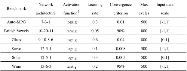
A total number of 42 experiments were set up for these 6 problems and the 7 weight initialization methods. Each experiment was carried out using a set of 100 initial weight vectors, selected by the corresponding method. The same network architecture was initialized with these vectors and trained using online BP. The network architecture and the training parameters, used in this arrangement, are reported in Table 1. These parameters are similar to those found by Thimm & Fiesler (1994).

a) Learning rate is the rate used by the vanilla BP online algorithm.

b) Convergence criterion is either the goal set for the minimization of the error function or the minimum percentage of the training patterns correctly classified by the network.

c) Max cycles denote the maximum number of BP cycles. During a cycle all train-ing patterns are presented to the network in random order and weights are up-dated after every training pattern. Training stops when Max cycles number is reached.

d) Input data scale indicates the interval used by all weight initialization algorithms except the Nguyen-Widrow algorithm, which scales input data values in the in-terval [−1,1].

Table 1: Architectures of networks and training parameters used for the Suite 1 of the experiments

Benchmark

Network Activation Learning Convergence Max Input data

architecture function† rate criterion cycles scale

Auto-MPG 7-3-1 logsig 0.3 0.01 500 [-1,1]

British Vowels 10-20-11 tansig 0.05 90% 800 [-1,1]

Glass 9-10-8-6 logsig 0.6 0.04 800 [0,1]

Servo 12-3-1 logsig 0.1 0.008 500 [-1,1]

Solar 12-5-1 logsig 0.3 0.005 500 [0,1]

Wine 13-6-3 tansig 0.2 95% 500 [-1,1]

4.1.2. Analysis of the Results

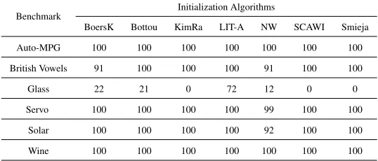
Tables 2, 3 and 4 report the experimental results on the benchmarks considered for the aforementioned performance measures. A quick look at these results shows that the proposed approach improves network performance for all parameters.

The comparison of the efficiency of the different initialization methods is based

Table 2: Convergence success results in 100 trials for the Suite 1 of the experiments

Benchmark

Initialization Algorithms

BoersK Bottou KimRa LIT-A NW SCAWI Smieja

Auto-MPG 100 100 100 100 100 100 100

British Vowels 91 100 100 100 91 100 100

Glass 22 21 0 72 12 0 0

Servo 100 100 100 100 99 100 100

Solar 100 100 100 100 92 100 100

Wine 100 100 100 100 100 100 100

on the statistical analysis of the results obtained. In order to evaluate the statistical sig-nificance of the observed performance one-way ANOVA (Green & Salkind, 2003) was used to test equality of means. ANOVA relies on three assumptions: independence, normality and homogeneity of variances of the samples. This procedure is robust with respect to violations of these assumptions except in the case of unequal variances with unequal sample sizes, which is true for the Glass benchmark as the larger group size is more than 1.5 times the size of the smaller group.

The validity of the normality assumption is omitted and Levene’s test for testing equality of variances is conducted, (Ramachandran & Tsokos, 2009). Homogeneity of variances is rejected for all cases by Levene’s test and so Tamhane’s posthoc procedure, (Ramachandran & Tsokos, 2009), is applied to perform multiple comparisons analysis of the samples. The significance level set for these tests isα = 0.05. The p-value (Sig.) indicated for each initialization method, concerns comparison with the proposed method and the mean value is marked with an∗ when equality of means is rejected

p-value<0.05. The analysis of the Glass benchmark results was performed pairwise between successful initialization methods using the Mann-Whitney test.

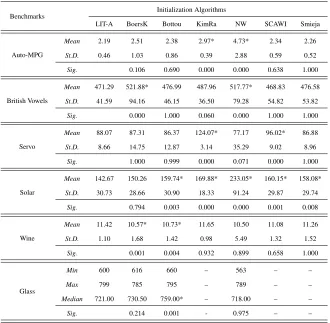
Table 3: Convergence rate results for the Suite 1 of the experiments

Benchmarks

Initialization Algorithms

LIT-A BoersK Bottou KimRa NW SCAWI Smieja

Auto-MPG

Mean 2.19 2.51 2.38 2.97* 4.73* 2.34 2.26

St.D. 0.46 1.03 0.86 0.39 2.88 0.59 0.52

Sig. 0.106 0.690 0.000 0.000 0.638 1.000

British Vowels

Mean 471.29 521.88* 476.99 487.96 517.77* 468.83 476.58

St.D. 41.59 94.16 46.15 36.50 79.28 54.82 53.82

Sig. 0.000 1.000 0.060 0.000 1.000 1.000

Servo

Mean 88.07 87.31 86.37 124.07* 77.17 96.02* 86.88

St.D. 8.66 14.75 12.87 3.14 35.29 9.02 8.96

Sig. 1.000 0.999 0.000 0.071 0.000 1.000

Solar

Mean 142.67 150.26 159.74* 169.88* 233.05* 160.15* 158.08*

St.D. 30.73 28.66 30.90 18.33 91.24 29.87 29.74

Sig. 0.794 0.003 0.000 0.000 0.001 0.008

Wine

Mean 11.42 10.57* 10.73* 11.65 10.50 11.08 11.26

St.D. 1.10 1.68 1.42 0.98 5.49 1.32 1.52

Sig. 0.001 0.004 0.932 0.899 0.658 1.000

Glass

Min 600 616 660 – 563 – –

Max 799 785 795 – 789 – –

Median 721.00 730.50 759.00* – 718.00 – –

Sig. 0.214 0.001 - 0.975 – –

∗_{denotes that the mean value of the initialization method is significantly different from the mean value of LIT-A} using the indicatedp-values (Sig.) computed by the posthoc analysis of the ANOVA results.

– denotes that the initialization method failed to meet the convergence criteria exceeding the maximum number of

cycles in all trials.

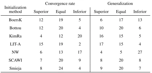
superior, equal or inferior performance when compared (pairwise comparisons) with all other methods regarding convergence rate and generalization. The advantage of-fered by the proposed method to achieve better convergence rate is manifested by these results. So, performance of a neural network when weights are initialized with the proposed method is superior in 42% of the cases. In 50% of the cases performance is the same with all other methods and only in 6% the proposed method delivers inferior performance to the training algorithm.

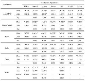
score when compared to the method of Kim and Ra proves to be better than all the other methods in all benchmarks, except in the case of the Glass benchmark, see Table 4. For the Glass benchmark the generalization performance seems to be better for the methods of Boers-Kuiper, Bottou and Nguyen-Widrow compared to our LIT-A method. How-ever, one should also take into account the number of successful experiments for each method. Generalization “achieved” by the proposed method is superior in 47% of the cases, while in 42% of the cases performance is the same with other methods and only in 11% of the cases the proposed method delivered inferior performance to the training algorithm. Only the method of Kim and Ra seems to give similar performance with the proposed LIT-Approach.

4.1.3. Non-parametric Statistical Analysis and Posthoc Procedures

In order to comply with reported best practice in the evaluation of the performance of neural networks, (Luengo et al., 2009; Garc´ıa et al., 2010; Derrac et al., 2011), we evaluated the statistical significance of the observed performance results applying the Friedman test. This test ranks the performance of a set ofkalgorithms and can detect a significant difference in the performance of at least two algorithms. More specifically, the Friedman test is a non-parametric statistical procedure similar to the parametric two-way ANOVA used to test if at least two of theksamples represent populations with different medians. The null hypothesisH0for Friedman‘s test states equality of medians between the populations while the alternative hypothesisH1is defined as the negation of the null hypothesis.

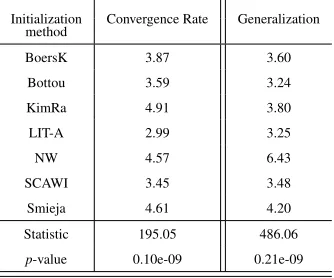
Table 6 uses two subtables to depict the average rankings computed through the above statistical test for the convergence rate and the generalization performance. At the bottom of each subtable we give the statistic of each test along with the correspond-ingp-value. Thep-values computed strongly suggest rejection of the null hypothesis at theα=0.05 level of significance. This means that the initialization algorithms have some pattern of larger and smaller scores (medians) among them i.e. there exist signif-icant differences among the considered algorithms.

Table 4: Generalization performance results for the Suite 1 of the experiments

Benchmarks

Initialization Algorithms

LIT-A BoersK Bottou KimRa NW SCAWI Smieja

Auto-MPG

Mean 0.0743 0.0750 0.0748 0.0738 0.0778* 0.0739 0.0741

St.D. 0.0041 0.0052 0.0047 0.0018 0.0073 0.0043 0.0041

Sig. 0.999 1.000 1.000 0.001 1.000 1.000

British Vowels

Mean 96.23% 93.72%* 96.29% 96.27% 94.52%* 95.86% 96.18%

St.D. 1.60% 2.85% 1.37% 1.18% 2.70% 1.81% 1.45%

Sig. 0.000 1.000 1.000 0.000 0.933 1.000

Servo

Mean 0.0792 0.0854* 0.0839* 0.0797* 0.0969* 0.0842* 0.0801*

St.D. 0.0010 0.0055 0.0045 0.0002 0.0145 0.0049 0.0020

Sig. 0.000 0.000 0.000 0.000 0.000 0.002

Solar

Mean 0.0924 0.0924 0.0919 0.0876* 0.1025* 0.0911 0.0917

St.D. 0.0040 0.0030 0.0030 0.0019 0.0107 0.0029 0.0034

Sig. 1.000 0.999 0.000 0.000 0.160 0.980

Wine

Mean 99.84% 98.98%* 99.38%* 99.80% 98.69%* 99.58% 99.40%*

St.D. 0.57% 1.20% 1.05% 0.64% 1.48% 0.93% 1.22%

Sig. 0.000 0.003 1.000 0.000 0.282 0.025

Glass

Min 59.62% 67.31% 65.38% - 65.38% -

-Max 71.15% 75.00% 75.00% - 75.00% -

-Median 65.38% 71.15%* 69.32%* - 69.23%* -

-Sig. 0.000 0.000 - 0.000 -

-* denotes that the mean value of the initialization method is significantly different from the mean value of LIT-A using

the indicatedp-values (Sig.) computed by the posthoc analysis of the ANOVA results.

– denotes that the initialization method failed to meet the convergence criteria exceeding the maximum number of cycles

in all trials.

trans-Table 5: Summary of pairwise comparisons score for each method for the Suite 1 of the experiments

Initialization

Convergence rate Generalization

method Superior Equal Inferior Superior Equal Inferior

BoersK 12 19 5 6 17 13

Bottou 12 20 4 10 20 6

KimRa 4 12 20 16 15 5

LIT-A 15 19 2 17 15 4

NW 6 13 17 4 5 27

SCAWI 7 20 9 8 20 8

Smieja 8 24 4 9 20 7

lates here to a smaller number of epochs and a better performance for generalization is taken to be a smaller classification or approximation error. So, the objective of the tests is minimization and in consequence the control procedure is automatically selected to be the algorithm with the lowest ranking score. This algorithm is LIT-Approach for both performance measures, see Table 6.

For the non-parametric test (Friedman) used we consider the ranking scores

com-Table 6: Average ranking achieved by the Friedman test (Suite 1 of the experiments)

Initialization Convergence Rate Generalization method

BoersK 3.75 4.69

Bottou 3.71 4.02

KimRa 5.15 3.33

LIT-A 3.15 2.81

NW 4.40 5.26

SCAWI 4.03 4.08

Smieja 3.82 3.82

Statistic 305.76 511.50

p-value 0.12e-09 0.23e-09

(2-tailed) corresponding to thez-statistic of each comparison is determined using nor-mal approximation and can be compared with some appropriate level of significance α.

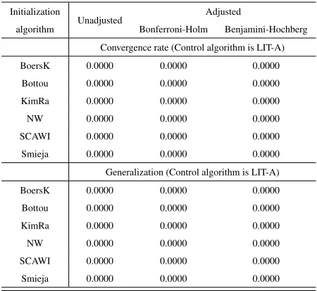
However, thesep-values are not suitable for multiple comparisons as they do not account for the Family-Wise Error Rate (FWER) produced by accumulation of Type I error in the case of a family of hypotheses associated with the multiple comparisons tests (Derrac et al., 2011). To cope with this matter, instead of using posthoc proce-dures to adjust the level of significanceα, we choose to compute the adjustedp-values (APVs) corresponding to the Holm (Bonferroni-Holm) and the Benjamini-Hochberg adjustment methods. Information on these adjustment methods can be found in R-Documentation (2013) and references cited therein. These APVs can be used to test the corresponding hypotheses i.e. to compare corresponding algorithms directly with any significance levelαand give a “metric” of how different these algorithms are (Lu-engo et al., 2009).

The unadjusted and the adjustedp-values for the pairwise comparison of the pro-posed algorithm with each one of the other methods are presented in Table 7 for both convergence rate and generalization. Note that the precision retained for thep-values given in this Table and all similar Tables hereafter is up to the fourth decimal digit. The adjustedp-values for the Friedman test in this Table show significant difference between the ranking of the LIT-Approach and the other methods for both convergence rate and generalization. This translates to an improvement of the LIT-Approch over all the other weight initialization algorithms.

The computations necessary for Table 6 as well as for all similar Tables hereafter in this paper were carried out using STATService (Parejo et al., 2012). Computations for Table 7 as well as for all similar Tables hereafter were executed using the R environ-ment for Statistical Data Analysis. Finally, it is worth noting that the results obtained using the non-parametric statistical analysis confirm those provided by ANOVA.

4.1.4. Comments and Remarks

Table 7:p-values of multiple comparisons (Suite 1 of the experiments) Initialization

Unadjusted Adjusted

algorithm Bonferroni-Holm Benjamini-Hochberg

Convergence rate (Control algorithm is LIT-A)

BoersK 0.0000 0.0000 0.0000

Bottou 0.0000 0.0000 0.0000

KimRa 0.0000 0.0000 0.0000

NW 0.0000 0.0000 0.0000

SCAWI 0.0000 0.0000 0.0000

Smieja 0.0000 0.0000 0.0000

Generalization (Control algorithm is LIT-A)

BoersK 0.0000 0.0000 0.0000

Bottou 0.0000 0.0000 0.0000

KimRa 0.0000 0.0000 0.0000

NW 0.0000 0.0000 0.0000

SCAWI 0.0000 0.0000 0.0000

Smieja 0.0000 0.0000 0.0000

method. In terms of convergence success (Table 2) the proposed method seems to con-tribute to the best score for the training algorithm. Moreover, the advantage offered by the proposed method to achieve better convergence rate is manifested by the results given in Table 3 and Table 5. Lastly, one may easily notice that in terms of general-ization performance the proposed method though marginally superior when compared, using ANOVA, to the Kim-Ra it proves to be better than all the other methods in all benchmarks, except the Glass benchmark, see Tables 4 and 5. These conclusions are strongly supported by the non-parametric statistical analysis with the Friedman test. Though these results are indicative and for comparison purposes, they provide signifi-cant evidence regarding the efficiency of the proposed method.

4.2. Function approximation

4.2.1. Setup of the Experiments

their method on a function approximation problem. The functions used as benchmarks are defined in the following paragraphs.

Function 1. The function for this benchmark is the one reported in the original paper of Nguyen & Widrow (1990),

y=0.5 sinπx2₁sin (2πx2).

The network used here, is a 3-layer (2-21-1) architecture with the hyperbolic tangent activation function for the hidden layer nodes as well as for the output node. A total of 625 (=25×25) points are randomly selected, using uniform ditribution, in the interval [−1,1]×[−1,1]. Among these points 450 are used for training and 175 for testing the network.

Function 2. The function considered here is a variant of the function considered in Yam & Chow (2000, 2001). This function is a mapping of eight input variables, taken in the interval [0,1], into three output ones defined by the following three equations:

y1 =(x1x2+x3x4+x5x6+x7x8)/4

y2 = √

(x1+x2+x3+x4+x5+x6+x7+x8)/8

y3 =(1−y1)1/3

For this benchmark, a 8-12-3 network architecture was used with logistic activation functions for nodes of the hidden and the output layer. A set of 75 patterns is formed by randomly sampling, with uniform distribution, values for the input variables and calculating output values. Among these input-output patterns, 50 are used for training the network and 25 for testing, as in Yam & Chow (2001).

Function 3. The function used here is a real-valued non-linear function of two vari-ables, taken in the interval [−1,1], defined by the formula:

y=sin (2πx1x2)/(2πx1x2).

tangent activation function. The training set is formed by taking 320 patterns of the total 400 (=20×20) that are randomly selected using uniform distribution. The rest 80 patterns constitute the test set.

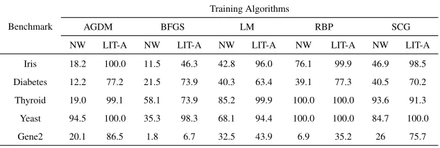
A total of 21 training experiments were executed for the above 3 functions and the 7 (LIT-A plus other six) weight initialization methods considered in this section. Each training experiment is made up of a hundred (100) initial weight vectors derived using one of the weight initialization methods. Networks in all experiments are trained using the Levenberg-Marquardt method (LM), (Hagan et al., 1996; Marquardt, 1963; Hagan & Menhaj, 1994). The performance goal for the network output error is set to 1.0e−04 forFunctions 1and2, and 1.0e−03 forFunction 3. If the performance goal is not met when a maximum number of 1000 epochs is reached then the training stops. The learning rate for all experiments ofFunction 1is set to 0.1 and 0.5 for the other two benchmarks. Results of the training experiments are reported in Tables 8 – 10 hereafter. For the benchmarksFunction1 andFunction3 LIT-A was applied using 1.5σxi for

the term sx_i. This choice is based on the assumption that the input data are approxi-mately normally distributed, and therefore sxi in the LIT-Approach was “roughly”

ap-proximated using 1.5σxiinstead of the third quartileQ3.

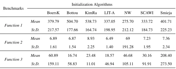
4.2.2. Analysis of the Results

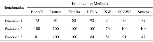
The results obtained regarding the performance measures set are shown in Tables 8–10. A rough observation of these results shows that the proposed LIT-Approach re-mains on top of the other methods as in the previous suite 1 concerning convergence rate (Table 9) while being among the best methods regarding convergence succes (Ta-ble 8) and generalization (Ta(Ta-ble 10).

Comparison between the performance of the different initialization methods, for

Table 8: Convergence success results for the Function Approximation benchmarks

Benchmarks

Initialization Methods

BoersK Bottou KimRa LIT-A NW SCAWI Smieja

Function 1 73 91 82 92 74 85 82

Function 2 100 100 100 100 76 100 100