BNSP: an R Package for fitting Bayesian semiparametric regression models and variable selection

Papageorgiou, Georgios (2018) BNSP: an R Package for fitting Bayesian

semiparametric regression models and variable selection. The R Journal 10

(2), pp. 526-548. ISSN 2073-4859.

Downloaded from:

Usage Guidelines:

Please refer to usage guidelines at

or alternatively

BNSP: an R Package for Fitting Bayesian

Semiparametric Regression Models and

Variable Selection

by Georgios Papageorgiou

Abstract The R packageBNSPprovides a unified framework for semiparametric location-scale

regression and stochastic search variable selection. The statistical methodology that the package is built upon utilizes basis function expansions to represent semiparametric covariate effects in the mean and variance functions, and spike-slab priors to perform selection and regularization of the estimated effects. In addition to the main function that performs posterior sampling, the package includes functions for assessing convergence of the sampler, summarizing model fits, visualizing covariate effects and obtaining predictions for new responses or their means given feature/covariate vectors.

Introduction

There are many approaches to non- and semi-parametric modeling. From a Bayesian perspective, Müller and Mitra(2013) provide a review that covers methods for density estimation, modeling of random effects distributions in mixed effects models, clustering, and modeling of unknown functions in regression models.

Our interest is on Bayesian methods for modeling unknown functions in regression models. In particular, we are interested in modeling both the mean and variance functions non-parametrically, as general functions of the covariates. There are multiple reasons why allowing the variance function to be a general function of the covariates may be important (Chan et al.,2006). Firstly, it can result in more realistic prediction intervals than those obtained by assuming constant error variance, or as Müller and Mitra(2013) put it, it can result in more honest representation of uncertainties. Secondly, it allows the practitioner to examine and understand which covariates drive the variance. Thirdly, it results in more efficient estimation of the mean function. Lastly, it produces more accurate standard errors of unknown parameters.

In the R (R Core Team,2016) packageBNSP(Papageorgiou,2018) we implemented Bayesian regression models with Gaussian errors and with mean and log-variance functions that can be mod-eled as general functions of the covariates. Covariate effects may enter the mean and log-variance functions parametrically or non-parametrically, with the nonparametric effects represented as linear combinations of basis functions. The strategy that we follow in representing unknown functions is to utilize a large number of basis functions. This allows for flexible estimation and for capturing true effects that are locally adaptive. Potential problems associated with large numbers of basis functions, such as over-fitting, are avoided in our implementation, and efficient estimation is achieved, by utilizing spike-slab priors for variable selection. A review of variable selection methods is provided by O’Hara and Sillanpää(2009).

The methods described here belong to the general class of models known as generalized additive models for location, scale, and shape (GAMLSS) (Rigby and Stasinopoulos,2005;Stasinopoulos and Rigby,2007) or the Bayesian analogue termed as BAMLSS (Umlauf et al.,2018) and implemented in packagebamlss(Umlauf et al.,2017). However, due to the nature of the spike-and-slab priors that we have implemented, in addition to flexible modeling of the mean and variance functions, the methods described here can also be utilized for selecting promising subsets of predictor variables in multiple regression models. The implemented methods fall in the general class of methods known as stochastic search variable selection (SSVS). SSVS has received considerable attention in the Bayesian literature and its applications range from investigating factors that affect individual’s happiness (George and McCulloch,1993), to constructing financial indexes (George and McCulloch,1997), and to gene mapping (O’Hara and Sillanpää,2009). These methods associate each regression coefficient, either a main effect or the coefficient of a basis function, with a latent binary variable that indicates whether the corresponding covariate is needed in the model or not. Hence, the joint posterior distribution of the vector of these binary variables can identify the models with the higher posterior probability.

R packages that are related toBNSPincludespikeSlabGAM(Scheipl,2016) that also utilizes SSVS methods (Scheipl,2011). A major difference between the two packages, however, is that whereas

spikeSlabGAMutilizes spike-and-slab priors for function selection,BNSPutilizes spike-and-slab

on boosting that can handle high-dimensional data (Mayr et al.,2012). Lastly, the R packagemgcv (Wood,2018) can also fit generalized additive models with Gaussian errors and integrated smoothness estimation, with implementations that can handle large datasets.

InBNSPwe have implemented functions for fitting such semi-parametric models, summarizing model fits, visualizing covariate effects and predicting new responses or their means. The main functions aremvrm,mvrm2mcmc,print.mvrm,summary.mvrm,plot.mvrm, andpredict.mvrm. A quick description of these functions follows. The first one,mvrm, returns samples from the posterior distri-butions of the model parameters, and it is based on an efficient Markov chain Monte Carlo (MCMC) algorithm in which we integrate out the coefficients in the mean function, generate the variable selection indicators in blocks (Chan et al.,2006), and choose the MCMC tuning parameters adaptively (Roberts and Rosenthal,2009). In order to minimize random-access memory utilization, posterior samples are not kept in memory, but instead written in files in a directory supplied by the user. The second function,mvrm2mcmc, reads-in the samples from the posterior of the model parameters and it creates an object of class"mcmc". This enables users to easily utilize functions from package coda(Plummer et al.,2006), including itsplotandsummarymethods for assessing convergence and for summarizing posterior distributions. Further, functionsprint.mvrmandsummary.mvrmprovide summaries of model fits, including models and priors specified, marginal posterior probabilities of term inclusion in the mean and variance models and models with the highest posterior probabilities. Functionplot.mvrmcreates plots of parametric and nonparametric terms that appear in the mean and variance models. The function can create two-dimensional plots by calling functions from the packageggplot2(Wickham,2009). It can also create static or interactive three-dimensional plots by calling functions from the packagesplot3D(Soetaert,2016) andthreejs(Lewis,2016). Lastly, function

predict.mvrmprovides predictions either for new responses or their means given feature/covariate vectors.

We next provide a detailed model description followed by illustrations on the usage of the package and the options it provides. Technical details on the implementation of the MCMC algorithm are provided in the Appendix. The paper concludes with a brief summary.

Mean-variance nonparametric regression models

Lety= (y1, . . . ,yn)>denote the vector of responses and letX= [x1, . . . ,xn]>andZ= [z1, . . . ,zn]> denote design matrices. The models that we consider express the vector of responses utilizing

Y=β01n+Xβ₁+e,

where1nis the usual n-dimensional vector of ones,β0is an intercept term,β₁is a vector of regression coefficients ande= (e1, . . . ,en)>is an n-dimensional vector of independent random errors. Each

e_i,i = 1, . . . ,n, is assumed to have a normal distribution,e_i ∼ N(0,σ_i2), with variances that are

modeled in terms of covariates. Letσ2= (σ₁2, . . . ,σ_n2)>. We model the vector of variances utilizing

log(σ2) =α01n+Zα1,

whereα0is an intercept term andα1is a vector of regression coefficients. Equivalently, the model for the variances can be expressed as

σ_i2=σ2exp(z_i>α1),i=1, . . . ,n, (1) whereσ2=exp(α0).

Let D(α) denote an n-dimensional, diagonal matrix with elements exp(z>_i α1/2),i = 1, . . . ,n. Then, the model that we consider may be expressed more economically as

Y=X∗β+e,

e∼N(0,σ2D2(α)), (2) whereβ= (β0,β>₁)>andX∗= [1n,X].

Locally adaptive models with a single covariate

Suppose that the observed dataset consists of triplets(yi,ui,wi),i=1, . . . ,n, where explanatory vari-ablesuandwenter flexibly the mean and variance models, respectively. To model the nonparametric effects ofuandwwe consider the following formulations of the mean and variance models

µ_i=β0+fµ(ui) =β0+ q1

∑

β_jφ_1j(u_i) =β0+x>_i β₁, (3)

log(σ_i2) =α0+fσ(wi) =α0+ q2

∑

αjφ2j(wi) =α0+z>_i α1. (4)

In the precedingx_i= (φ11(ui), . . . ,φ1q1(ui))>andzi= (φ21(wi), . . . ,φ2q2(wi))>are vectors of basis

functions andβ₁= (β1, . . . ,βq1)>andα1= (α1, . . . ,αq2)>are the corresponding coefficients.

In packageBNSPwe implemented two sets of basis functions. Firstly, radial basis functions

B1=φ1(u) =u,φ2(u) =||u−ξ1||2log

||u−ξ1||2

, . . . ,

φq(u) =||u−ξq−1||2log

||u−ξq−1||2

, (5)

where||u||denotes the Euclidean norm ofuandξ1, . . . ,ξq−1are the knots that within packageBNSP are chosen as the quantiles of the observed values of explanatory variableu, withξ1 = min(ui),

ξq−1=max(ui)and the remaining knots chosen as equally spaced quantiles betweenξ1andξq−1. Secondly, we implemented thin plate splines

B2=φ1(u) =u,φ2(u) = (u−ξ1)+, . . . ,φq(u) = (u−ξq)+ ,

where(a)+=max(a, 0)and the knotsξ₁, . . . ,ξ_q−1are determined as above.

In addition,BNSPsupports the smooth constructors from packagemgcv(e.g., the low-rank thin plate splines, cubic regression splines, P-splines, their cyclic versions, and others). Examples on how these smooth terms are used withinBNSPare provided later in this paper.

Locally adaptive models for the mean and variance functions are obtained utilizing the method-ology developed byChan et al.(2006). Considering the mean function, local adaptivity is achieved by utilizing a large number of basis functions,q1. Over-fitting, and problems associated with it, is avoided by allowing positive prior probability that the regression coefficients are exactly zero. The latter is achieved by defining binary variablesγj,j=1, . . . ,q1, that take valueγj =1 ifβj 6=0 and

γ_j=0 ifβ_j=0. Hence, vectorγ= (γ₁, . . . ,γq1)>determines which terms enter the mean model. The

vector of indicatorsδ= (δ1, . . . ,δq2)>for the variance function is defined analogously.

Given vectorsγandδ, the heteroscedastic, semiparametric model (2) can be written as

Y=X∗_γβ_γ+e,

e∼N(0,σ2D2(α_δ)),

whereβ_γconsisting of all non-zero elements ofβ₁andX∗γconsists of the corresponding columns of

X∗. Subvectorαδis defined analogously.

We note that, as was suggested byChan et al.(2006), we work with mean corrected columns in the design matricesXandZ, both in this paper and in theBNSPimplementation. We remove the mean

from all columns in the design matrices except those that correspond to categorical variables.

Prior specification for models with a single covariate

Let ˜X=D(α)−1X∗. The prior forβ_γis specified as (Zellner,1986)

β_γ|cβ,σ2,γ,α,δ∼N(0,cβσ2(X˜ > γX˜γ)−1).

Further, the prior forαδis specified as

αδ|cα,δ∼N(0,cαI).

from which the joint prior is obtained as

P(γ|πµ) =π N(γ)

µ (1−πµ)q1−N(γ), whereN(γ) =∑q_j=1₁γ_j.

Similarly, for the indicatorsδ_jwe specify independent priorsP(δ_j=1|πσ) =πσ,j=1, . . . ,q2. It follows that the joint prior is

P(δ|πσ) =π N(δ)

σ (1−πσ)q2−N(δ), whereN(δ) =∑q_j=2₁δj.

We specify inverse Gamma priors forcβandcαand Beta priors forπµandπσ

cβ∼IG(aβ,bβ),cα∼IG(aα,bα),

πµ∼Beta(cµ,dµ),πσ∼Beta(cσ,dσ). (6) Lastly, forσ2we consider inverse Gamma and half-normal priors

σ2∼IG(aσ,bσ)and|σ| ∼N(0,φ2σ). (7)

Extension to bivariate covariates

It is straightforward to extend the methodology described earlier to allow fitting of flexible mean and variance surfaces. In fact, the only modification required is in the basis functions and knots. For fitting surfaces, in packageBNSPwe implemented radial basis functions

B3=

n

φ1(u) =u1,φ2(u) =u2,φ3(u) =||u−ξ₁||2log

||u−ξ₁||2

, . . . ,

φq(u) =||u−ξ_q−2||2log

||u−ξ_q−2||2 o

.

We note that the prior specification presented earlier for fitting flexible functions remains unchained for fitting flexible surfaces. Further, for fitting bivariate or higher order functions,BNSPalso supports smooth constructorss,te, andtifrommgcv.

Extension to additive models

In the presence of multiple covariates, the effects of which may be modeled parametrically or semi-parametrically, the mean model in (3) is extended to the following

µ_i=β₀+u>_ipβ+ K1

∑

fµ,k(uik),i=1, . . . ,n,

whereu_ip includes the covariates the effects of which are modeled parametrically, βdenotes the corresponding effects, and fµ,k(uik),k=1, . . . ,K1, are flexible functions of one or more covariates expressed as

fµ,k(uik) = q1k

∑

βkjφ1kj(uik),

whereφ1kj,j=1, . . . ,q1kare the basis functions used in thekth component,k=1, . . . ,K1. Similarly, the variance model (4), in the presence of multiple covariates, is expressed as

log(σ_i2) =α0+w>_ipα+ K2

∑

fσ,k(wik),i=1, . . . ,n,

where

fσ,k(wik) = q2k

∑

α_kjφ_2kj(w_ik).

γ_k= (γ_k1, . . . ,γ_kq1k)>,k=1, . . . ,K₁, andδ_k= (δ_k1, . . . ,δ_kq2k)>,k=1, . . . ,K2. Here, vectorsγ_kandδ_k determine which basis functions appear infµ,kandfσ,krespectively.

The model that we implemented in packageBNSPspecifies independent priors for the indicators variablesγ_kjasP(γ_kj=1|πµk) =πµk,j=1, . . . ,q1k. From these, the joint prior follows

P(γ_k|πµk) =π

N(γk)

µk (1−πµk)q1k−N(γk),

whereN(γ_k) =∑q_j=1k₁γ_kj.

Similarly, for the indicatorsδ_kjwe specify independent priorsP(δ_kj=1|πσk) =πσk,j=1, . . . ,q2k.

It follows that the joint prior is

P(δ_k|πσk) =π

N(δk)

σk (1−πσk)q2k−N(δk),

whereN(δk) =∑qj=2k1δkj.

We specify the following independent priors for the inclusion probabilities.

πµk ∼Beta(cµk,dµk),k=1, . . . ,K1 πσk ∼Beta(cσk,dσk),k=1, . . . ,K2. (8)

The rest of the priors are the same as those specified for the single covariate models.

Usage

In this section we provide results on simulation studies and real data analyses. The purpose is twofold: firstly we point out that the package works well and provides the expected results (in simulation studies) and secondly we illustrate the options that the users ofBNSPhave.

Simulation studies

Here we present results from three simulations studies, involving one, two, and multiple covariates. For the majority of these simulation studies, we utilize the same data-generating mechanisms as those presented byChan et al.(2006).

Single covariate case

We consider two mechanisms that involve a single covariate that appears in both the mean and variance model. Denoting the covariate byu, the data-generating mechanisms are the normal model Y∼N{µ(u),σ2(u)}with the following mean and standard deviation functions:

1. µ(u) =2u,σ(u) =0.1+u,

2. µ(u) =N(u,µ=0.2,σ2=0.004) +N(u,µ=0.6,σ2=0.1) /4, σ(u) =N(u,µ=0.2,σ2=0.004) +N(u,µ=0.6,σ2=0.1) /6.

We generate a single dataset of sizen=500 from each mechanism, where variableuis obtained from the uniform distribution,u∼Unif(0, 1). For instance, for obtaining a dataset from the first mechanism we use

> mu <- function(u) {2 * u} > stdev <- function(u) {0.1 + u} > set.seed(1)

> n <- 500

> u <- sort(runif(n))

> y <- rnorm(n, mu(u), stdev(u)) > data <- data.frame(y, u)

Above we specified the seed value to be one, and we do so in what follows, so that our results are replicable.

To the generated dataset we fit a special case of the model that we presented, where the mean and variance functions in (3) and (4) are specified as

µ=β0+fµ(u) =β0+ q1

∑

β_jφ_1j(u) and log(σ2) =α0+fσ(u) =α0+ q2

∑

withφdenoting the radial basis functions presented in (5). Further, we chooseq₁ =q2 =21 basis

functions or, equivalently, 20 knots. Hence, we haveφ1j(u) =φ2j(u),j=1, . . . , 21, which results in identical design matrices for the mean and variance models. In R, the two models are specified using

> model <- y ~ sm(u, k = 20, bs = "rd") | sm(u, k = 20, bs = "rd")

The above formula (Zeileis and Croissant,2010) specifies the response, mean and variance models. Smooth terms are specified utilizing functionsm, that takes as input the covariateu, the selected number of knots and the selected type of basis functions.

Next we specify the hyper-parameter values for the priors in (6) and (7). The default prior forcβis inverse Gamma withaβ=0.5,bβ=n/2 (Liang et al.,2008). For parametercαthe default prior is a non-informative but proper inverse Gamma withaα=bα=1.1. Concerningπµandπσ, the default priors are uniform, obtained by settingcµ=dµ=1 andcσ=dσ=1. Lastly, the default prior for the error standard deviation is the half-normal with varianceφ2_σ=2,|σ| ∼N(0, 2).

We choose to run the MCMC sampler for 10, 000 iterations and discard the first 5, 000 as burn-in. Of the remaining 5, 000 samples we retain 1 of every 2 samples, resulting in 2, 500 posterior samples. Further, as mentioned above, we set the seed of the MCMC sampler equal to one. Obtaining posterior samples is achieved by a function call of the form

> DIR <- getwd()

> m1 <- mvrm(formula = model, data = data, sweeps = 10000, burn = 5000, + thin = 2, seed = 1, StorageDir = DIR,

+ c.betaPrior = "IG(0.5,0.5*n)", c.alphaPrior = "IG(1.1,1.1)",

+ pi.muPrior = "Beta(1,1)", pi.sigmaPrior = "Beta(1,1)", sigmaPrior = "HN(2)")

Samples from the posteriors of the model parameters{β,γ,α,δ,c_β,cα,σ2}are written in seven separate files which are stored in the directory specified by argumentStorageDir. If a storage directory is not specified, then functionmvrmreturns an error message, as without these files there will be no output to process. Furthermore, the last two lines of the above function call show the specified priors, which arecβ∼ IG(0.5,n/2),cα ∼IG(1.1, 1.1),πµ ∼Beta(1, 1),πσ ∼Beta(1, 1)and|σ| ∼ N(0, 2), respectively. As we mentioned above, these priors are the default ones, and hence the same function call can be achieved without specifying the last two lines. Here we display the priors in order to describe how users can specify their own priors. For parameterscβandcαonly inverse Gamma priors are available, with parameters that can be specified by the user in the intuitive way. For instance, the priorcβ∼IG(1.01, 1.01)can be specified in functionmvrmby usingc.betaPrior = "IG(1.01,1.01)". The second parameter of the prior forcβcan be a function of the sample sizen(but only symboln would work here), so for instancec.betaPrior = "IG(1,0.4*n)"is another acceptable specification. Further, Beta priors are available for parametersπµandπσwith parameters that can be specified by the user again in the intuitive way. Lastly, two priors are available for the error variance. These are the default half-normal and the inverse Gamma. For instance,sigmaPrior = "HN(5)"defines

|σ| ∼N(0, 5)as the prior whilesigmaPrior = "IG(1.1,1.1)"definesσ2∼IG(1.1, 1.1)as the prior.

Functionmvrm2mcmcreads in posterior samples from the files that the call to functionmvrmgenerated and creates an object of class"mcmc". Hence, for summarizing posterior distributions and for assessing convergence, functionssummaryandplotfrom packagecodacan be used. As an example, here we read in the samples from the posterior ofβand summarize the posterior usingsummary. For the sake of economizing space, only the part of the output that describes the posteriors ofβ0,β1, andβ2is shown below:

> beta <- mvrm2mcmc(m1, "beta")

> summary(beta)

Iterations = 5001:9999 Thinning interval = 2 Number of chains = 1

Sample size per chain = 2500

1. Empirical mean and standard deviation for each variable, plus standard error of the mean:

5000 6000 7000 8000 9000 10000

0.90

1.00

Iterations

Trace of (Intercept)

0.90 0.92 0.94 0.96 0.98 1.00

0

60

Density of (Intercept)

N = 2500 Bandwidth = 0.0006888

5000 6000 7000 8000 9000 10000

1.4

2.2

Iterations

Trace of u

1.4 1.6 1.8 2.0 2.2 2.4

0

30

Density of u

N = 2500 Bandwidth = 0.001937

5000 6000 7000 8000 9000 10000

−0.2

0.4

Iterations

Trace of sm(u).1 Density of sm(u).1

0

10

−1.281334 −0.281334 0.168114 0.613418

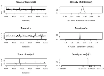
Figure 1:Trace and density plots for the regression coefficientsβ0,β1andβ2of the first simulated

example. Parametersβ1andβ2are the coefficients of the first two basis functions, denoted by “u” and “sm(u).1”. Plots for coefficientsβ3, . . . ,β21are omitted as they follow a very similar pattern to that

seen forβ2(i.e., most of the time they take value zero but with random spikes away from zero).

2. Quantiles for each variable:

2.5% 25% 50% 75% 97.5% (Intercept) 0.946 0.9513 0.9533 0.9554 0.960 u 1.833 1.8565 1.8614 1.8682 1.923 sm(u).1 0.000 0.0000 0.0000 0.0000 0.000

Further, we may obtain a plot using

> plot(beta)

Figure1shows the first three of the plots created by functionplot. These are the plots of the samples from the posteriors of coefficientsβ0,β1andβ2. As we can see from both the summary and Figure1, only the first two coefficients have posteriors that are not centered around zero.

Returning to the functionmvrm2mcmc, it requires two inputs. These are an object of class"mvrm"and the name of the file to be read in R. For the parameters in the current model{β,γ,α,δ,c_β,cα,σ2}the corresponding file names are ‘beta’, ‘gamma’, ‘alpha’, ‘delta’, ‘cbeta’, ‘calpha’, and ‘sigma2’ respectively.

Summaries ofmvrmfits may be obtained utilizing functionsprint.mvrmandsummary.mvrm. The methodprinttakes as input an object of class"mvrm". It returns basic information of the model fit, as shown below:

> print(m1)

Call:

mvrm(formula = model, data = data, sweeps = 10000, burn = 5000,

thin = 2, seed = 1, StorageDir = DIR, c.betaPrior = "IG(0.5,0.5*n)", c.alphaPrior = "IG(1.1,1.1)", pi.muPrior = "Beta(1,1)",

pi.sigmaPrior = "Beta(1,1)", sigmaPrior = "HN(2)")

2500 posterior samples

u sm(u).1 sm(u).2 sm(u).3 sm(u).4 sm(u).5 sm(u).6 sm(u).7 1.0000 0.0040 0.0036 0.0032 0.0084 0.0036 0.0044 0.0028 sm(u).8 sm(u).9 sm(u).10 sm(u).11 sm(u).12 sm(u).13 sm(u).14 sm(u).15 0.0060 0.0020 0.0060 0.0036 0.0056 0.0056 0.0036 0.0052 sm(u).16 sm(u).17 sm(u).18 sm(u).19 sm(u).20

0.0060 0.0044 0.0056 0.0044 0.0052

Variance model - marginal inclusion probabilities

u sm(u).1 sm(u).2 sm(u).3 sm(u).4 sm(u).5 sm(u).6 sm(u).7 1.0000 0.6072 0.5164 0.5808 0.5488 0.6760 0.5320 0.6336 sm(u).8 sm(u).9 sm(u).10 sm(u).11 sm(u).12 sm(u).13 sm(u).14 sm(u).15 0.6936 0.6708 0.5996 0.4816 0.4912 0.3728 0.6268 0.5688 sm(u).16 sm(u).17 sm(u).18 sm(u).19 sm(u).20

0.5872 0.6528 0.4428 0.6900 0.5356

The function returns a matched call, the number of posterior samples obtained, and marginal inclusion probabilities of the terms in the mean and variance models.

Whereas the output of theprintmethod focuses on marginal inclusion probabilities, the output of thesummarymethod focuses on the most frequently visited models. It takes as input an object of class

"mvrm"and the number of (most frequently visited) models to be displayed, which by default is set to

nModels = 5. Here to economize space we setnModels = 2. The information returned by thesummary

method is shown below

> summary(m1, nModels = 2)

Specified model for the mean and variance:

y ~ sm(u, k = 20, bs = "rd") | sm(u, k = 20, bs = "rd")

Specified priors:

[1] c.beta = IG(0.5,0.5*n) c.alpha = IG(1.1,1.1) pi.mu = Beta(1,1) [4] pi.sigma = Beta(1,1) sigma = HN(2)

Total posterior samples: 2500 ; burn-in: 5000 ; thinning: 2

Files stored in /home/papgeo/1/

Null deviance: 1299.292 Mean posterior deviance: -88.691

Joint mean/variance model posterior probabilities:

mean.u mean.sm.u..1 mean.sm.u..2 mean.sm.u..3 mean.sm.u..4 mean.sm.u..5

1 1 0 0 0 0 0

2 1 0 0 0 0 0

mean.sm.u..6 mean.sm.u..7 mean.sm.u..8 mean.sm.u..9 mean.sm.u..10

1 0 0 0 0 0

2 0 0 0 0 0

mean.sm.u..11 mean.sm.u..12 mean.sm.u..13 mean.sm.u..14 mean.sm.u..15

1 0 0 0 0 0

2 0 0 0 0 0

mean.sm.u..16 mean.sm.u..17 mean.sm.u..18 mean.sm.u..19 mean.sm.u..20 var.u

1 0 0 0 0 0 1

2 0 0 0 0 0 1

var.sm.u..1 var.sm.u..2 var.sm.u..3 var.sm.u..4 var.sm.u..5 var.sm.u..6

1 1 1 1 1 1 1

2 1 0 1 1 1 1

var.sm.u..7 var.sm.u..8 var.sm.u..9 var.sm.u..10 var.sm.u..11 var.sm.u..12

1 1 1 1 0 1 0

2 1 1 1 1 1 1

var.sm.u..13 var.sm.u..14 var.sm.u..15 var.sm.u..16 var.sm.u..17 var.sm.u..18

1 1 1 1 1 1 1

2 0 1 1 1 1 0

var.sm.u..19 var.sm.u..20 freq prob cumulative

1 1 1 141 5.64 5.64

2 1 0 120 4.80 10.44

2 models account for 10.44% of the posterior mass

Firstly, the method provides the specified mean and variance models and the specified priors. This is followed by information about the MCMC chain and the directory where files have been stored. In addition, the function provides the null and the mean posterior deviance. Finally, the function provides the specification of the joint mean/variance models that were visited most often during MCMC sampling. This specification is in terms of a vector of indicators, each consisting of zeros and ones, that show which terms are in the mean and variance model. To make clear which terms pertain to the mean and which to the variance function, we have preceded the names of the model terms by “mean.” or “var.”. In the above output, we see that the most visited model specifies a linear mean model (only the linear term is included in the model) while the variance model includes twelve terms. See also Figure2.

We next describe the functionplot.mvrmwhich creates plots of terms in the mean and variance functions. Two calls to theplotmethod can be seen in the code below. Argumentxexpects an object of class"mvrm", as created by a call to the functionmvrm. Themodelargument may take on one of three possible values:"mean","stdev", or"both", specifying the model to be visualized. Further, theterm

argument determines the term to be plotted. In the current example there is only one term in each of the two models which leaves us with only one choice,term = "sm(u)". Equivalently,termmay be specified as an integer,term = 1. Iftermis left unspecified, then, by default, the first term in the model is plotted. For creating two-dimensional plots, as in the current example, theplotmethod utilizes the packageggplot2. Users ofBNSPmay add their own options to plots via the argumentplotOptions. The code below serves as an example.

> x1 <- seq(0, 1, length.out = 30)

> plotOptionsM <- list(geom_line(aes_string(x = x1, y = mu(x1)), col = 2, alpha = 0.5, + lty = 2), geom_point(data = data, aes(x = u, y = y)))

> plot(x = m1, model = "mean", term = "sm(u)", plotOptions = plotOptionsM, + intercept = TRUE, quantiles = c(0.005, 0.995), grid = 30)

> plotOptionsV = list(geom_line(aes_string(x = x1, y = stdev(x1)), col = 2,

+ alpha = 0.5, lty = 2))

> plot(x = m1, model = "stdev", term = "sm(u)", plotOptions = plotOptionsV, + intercept = TRUE, quantiles = c(0.05, 0.95), grid = 30)

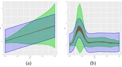
The resulting plots can be seen in Figure2, panels (a) and (b). Panel (a) displays the simulated dataset, showing the expected increase in both the mean and variance with increasing values of the covariateu. Further, we see the posterior mean ofµ(u) =β0+fµ(u) =β0+∑21j=1βjφ1j(u)evaluated over a grid of 30 values ofu, as specified by the (default)grid = 30option forplot. For each sampleβ(s),s=1, . . . ,S, from the posterior ofβ, and for each value ofuover the grid of 30 values,

uj,j =1, . . . , 30, theplotmethod computesµ(uj)(s) = β₀(s)+∑21_j=1β(_js)φ1j(uj). The default option intercept = TRUEspecifies that the interceptβ0is included in the computation, but it may be removed by settingintercept = FALSE. The posterior means are computed by the usual ¯µ(u_j) =S−1∑_sµ(u_j)(s)

and are plotted with solid (blue-color) line. By default, the function displays 80% point-wise credible intervals (CI). In Figure2, panel (a) we have plotted 99% CIs, as specified by optionquantiles = c(0.005,0.995). This option specifies that for each valueuj,j=1, . . . , 30, on the grid, 99% CIs for

µ(uj)are computed by the 0.5% and 99.5% quantiles of the samplesµ(uj)(s),s=1, . . . ,S. Plots without credible intervals may be obtained by settingquantiles = NULL.

Figure 2, panel (b) displays the posterior mean of the standard deviation function σ(u) = σexp{∑q_j=2₁αjφ2j(u)/2}. The details are the same as for the plot of the mean function, so here we briefly mention a difference: optionintercept = TRUEspecifies thatσis included in the calculation. It may be

removed by settingintercept = FALSE, which will result in plots ofσ(u)∗=exp{∑_jq₌2₁α_jφ_2j(u)/2}.

We use the second simulated dataset to show how thesconstructor from the packagemgcvmay be used. In our example, we usesto specify the model:

> model <- y ~ s(u, k = 15, bs = "ps", absorb.cons=TRUE) | + s(u, k = 15, bs = "ps", absorb.cons=TRUE)

FunctionBNSP::scalls in turnmgcv::sandmgcv::smoothCon. All options of the last two functions may be passed toBNSP::s. In the example above we used optionsk,bs, andabsorb.cons.

The remaining R code for the second simulated example is precisely the same as the one for the first example, and hence omitted. Results are shown in Figure2, panels (c) and (d).

● ●●● ●● ● ●● ● ● ●● ● ● ● ● ● ● ● ● ● ● ● ● ● ● ● ● ● ● ● ● ● ● ●● ● ● ● ● ● ● ● ● ● ● ● ●● ● ● ● ● ● ● ● ● ● ● ● ● ● ● ● ● ● ● ● ● ● ● ● ● ● ● ● ● ● ● ● ● ● ● ● ● ● ● ● ● ● ● ● ● ● ● ● ● ● ● ● ● ● ● ● ● ● ● ● ● ● ● ●● ● ● ● ● ● ● ● ● ● ● ● ● ● ● ● ● ● ● ● ● ● ● ● ● ● ● ● ● ● ● ● ● ● ● ● ● ● ● ● ● ● ●●● ● ● ● ● ● ● ● ● ● ● ● ● ● ● ● ● ● ● ● ● ● ● ● ● ● ● ● ● ● ● ● ● ● ● ● ● ● ● ● ● ● ● ● ● ● ● ● ● ● ● ● ● ● ● ● ● ● ● ● ● ● ● ● ● ● ● ● ● ● ● ● ● ● ● ● ● ● ● ● ● ● ● ● ● ● ● ● ● ● ● ● ● ● ● ● ● ● ● ● ● ● ● ● ● ● ● ● ● ● ● ● ● ● ● ● ● ● ● ● ● ● ● ● ● ● ● ● ● ● ● ● ●● ● ● ● ● ● ● ● ● ●● ● ● ● ● ● ● ● ● ● ● ● ● ● ● ● ●● ● ● ● ●● ● ● ● ● ● ● ● ● ● ● ● ● ● ● ● ● ● ● ● ● ● ● ● ● ● ● ● ● ● ● ● ● ● ● ● ● ● ● ● ● ● ● ● ● ● ● ● ● ● ●● ● ● ● ● ● ● ● ● ● ● ● ● ● ● ● ● ● ● ● ● ● ● ● ● ●● ● ● ● ● ● ● ● ● ● ● ● ● ● ● ● ● ● ● ● ● ● ● ● ● ● ● ● ● ● ● ● ● ● ● ● ● ● ● ● ● ● ● ● ● ● ● ● ●● ● ● ● ● ● ● ● ● ● ● ● ● ● ● ● ● ● ● ● ● ● ● ● ● ● ● ● ● ● ● ● ● ● ● ● ● ● ● ● ● ● ● ● ● ● ● ● ● ● ● ● −1 0 1 2 3 4

0.00 0.25 0.50 0.75 1.00

u sm(u) mean 0.4 0.8 1.2 1.6

0.00 0.25 0.50 0.75 1.00

u sm(u) st dev (a) (b) ● ●●●●● ● ●●● ● ●● ● ● ● ● ● ● ● ● ● ● ● ● ● ● ● ● ● ● ● ● ● ● ● ● ● ● ● ● ● ● ● ● ● ● ● ● ● ● ● ● ● ● ● ● ● ● ● ● ● ● ● ● ● ● ● ● ● ● ● ● ● ● ● ● ● ● ● ● ● ● ● ● ● ● ● ● ● ● ● ● ● ● ● ● ● ● ● ● ● ● ● ● ● ● ● ● ● ● ● ● ● ● ● ● ● ● ● ● ● ● ● ● ● ● ● ● ● ● ● ● ● ● ● ● ● ● ● ● ● ● ● ● ● ● ● ● ●● ● ●●●●●● ● ● ● ● ● ● ● ● ● ● ● ● ● ● ● ● ● ● ● ● ● ● ● ● ● ● ● ● ● ● ● ● ● ● ● ● ● ● ● ● ● ● ● ●● ● ● ● ● ● ● ● ● ● ● ● ●● ● ● ● ● ● ● ● ● ● ● ● ● ● ● ● ● ●● ● ● ● ● ● ● ● ● ● ● ● ● ● ● ● ● ● ● ● ● ● ● ● ● ● ● ● ● ● ● ● ● ● ● ● ● ● ● ● ● ● ● ● ● ● ● ● ● ● ● ● ● ● ● ● ●● ●● ● ● ● ● ● ● ●● ● ● ● ● ● ● ● ● ● ● ● ● ● ● ● ●● ● ● ● ●● ● ●●● ● ● ● ● ● ● ● ● ● ● ●● ● ● ● ● ● ● ● ●● ● ● ● ● ● ● ● ● ● ● ● ● ● ● ● ● ● ● ● ● ● ● ● ● ●● ● ● ● ● ● ● ● ● ● ● ● ● ● ● ● ● ● ● ● ● ● ● ● ● ●●● ● ● ● ● ● ● ● ● ● ● ● ●● ● ● ● ● ● ● ● ● ● ● ● ● ● ● ● ● ● ● ●● ● ●● ● ● ● ● ● ● ● ● ● ● ●● ● ● ● ●● ● ●● ● ● ●● ● ● ● ● ● ● ● ● ● ● ● ● ● ● ● ● ● ● ●● ● ● ● ● ● ● ● ● ● ● ● ● ● ● ● ● ● ● ● −1 0 1 2 3 4

0.00 0.25 0.50 0.75 1.00

u s(u) mean 0.0 0.5 1.0 1.5

0.00 0.25 0.50 0.75 1.00

u

s(u)

st dev

(c) (d)

Figure 2:Results from the single covariate simulated examples. The column on the left-hand side

displays the generated data points and posterior means of the estimated effect along with 99% CIs. The column on the right-hand side displays the posterior mean of the estimated standard deviation function along with 90% CIs. In all panels, the truth is represented by dashed (red color) lines, the posterior means by solid (blue color) lines, and the CIs by gray color.

The following code shows how credible and prediction intervals can be obtained for a sequence of covariate values stored inx1

> x1 <- seq(0, 1, length.out = 30)

> p1 <- predict(m1, newdata = data.frame(u = x1), interval = "credible") > p2 <- predict(m1, newdata = data.frame(u = x1), interval = "prediction")

where the first argument in thepredictmethod is a fittedmvrmmodel, the second one is a data frame containing the feature vectors at which predictions are to be obtained and the last one defines the type of interval to be created. We applied thepredictmethod to the two simulated datasets. To each of those datasets we fitted two models: the first one is the one we saw earlier, where both the mean and variance are modeled in terms of covariates, while the second one ignores the dependence of the variance on the covariate. The latter model is specified in R using

> model <- y ~ sm(u, k = 20, bs = "rd") | 1

Results are displayed in Figure3. Each of the two figures displays a credible interval and two prediction intervals. The figure emphasizes a point that was discussed in the introductory section, that modeling the variance in terms of covariates can result in more realistic prediction intervals. The same point was recently discussed byMayr et al.(2012).

Bivariate covariate case

Interactions between two predictors can be modeled by appropriate specification of either the built-in

0 2 4

0.00 0.25 0.50 0.75 1.00

x1

fit

0 1 2 3 4

0.00 0.25 0.50 0.75 1.00

x1

fit

(a) (b)

Figure 3:Predictions results from the first two simulated datasets. Each panel displays a credible

interval and two prediction intervals, one obtained using a model that recognizes the dependence of the variance on the covariate and one that ignores it.

Letu= (u1,u2)>denote a bivariate predictor. The data-generating mechanism that we consider is

y(u)∼N{µ(u),σ2(u)},

µ(u) =0.1+N(u,µ₁,Σ1) +N(u,µ₂,Σ2),

σ2(u) =0.1+{N(u,µ₁,Σ1) +N(u,µ₂,Σ2)}/2,

µ₁= _0.25

0.75

,Σ1=

_{0.03 0.01} 0.01 0.03

,µ₂= _0.65

0.35

,Σ2=

_{0.09 0.01} 0.01 0.09

.

As before,u1 andu2are obtained independently from uniform distributions on the unit interval. Further, the sample size is set ton=500.

In R, we simulate data from the above mechanism using

> mu1 <- matrix(c(0.25, 0.75))

> sigma1 <- matrix(c(0.03, 0.01, 0.01, 0.03), 2, 2) > mu2 <- matrix(c(0.65, 0.35))

> sigma2 <- matrix(c(0.09, 0.01, 0.01, 0.09), 2, 2) > mu <- function(x1, x2) {x <- cbind(x1, x2);

+ 0.1 + dmvnorm(x, mu1, sigma1) + dmvnorm(x, mu2, sigma2)} > Sigma <- function(x1, x2) {x <- cbind(x1, x2);

+ 0.1 + (dmvnorm(x, mu1, sigma1) + dmvnorm(x, mu2, sigma2)) / 2} > set.seed(1)

> n <- 500 > w1 <- runif(n) > w2 <- runif(n) > y <- vector()

> for (i in 1:n) y[i] <- rnorm(1, mean = mu(w1[i], w2[i]),

+ sd = sqrt(Sigma(w1[i], w2[i])))

> data <- data.frame(y, w1, w2)

We fit a model with mean and variance functions specified as

µ(u) =β0+ 12

∑

12

∑

βj1,j2φ1j1,j2(u), log(σ2(u)) =α0+

12

∑

12

∑

αj1,j2φ2j1,j2(u).

The R code that fits the above model is

> Model <- y ~ sm(w1, w2, k = 10, bs = "rd") | sm(w1, w2, k = 10, bs = "rd") > m2 <- mvrm(formula = Model, data = data, sweeps = 10000, burn = 5000, thin = 2, + seed = 1, StorageDir = DIR)

As in the univariate case, convergence assessment and univariate posterior summaries may be obtained by using functionmvrm2mcmcin conjunction with functionsplot.mcmcandsummary.mcmc. Further, summaries of themvrmfits may be obtained using functionsprint.mvrmandsummary.mvrm. Plots of the bivariate effects may be obtained using functionplot.mvrm. This is shown below, where argumentplotOptionsutilizes the packagecolorspace(Zeileis et al.,2009).

w1 w2

sm(w1,w2)

mean

0 1 2 3 4 5

w1 w2

sm(w1,w2)

st dev

0.4 0.6 0.8 1.0 1.2 1.4 1.6

(a) (b)

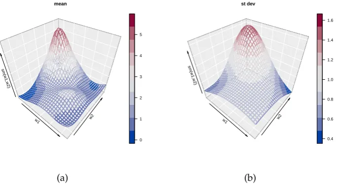
Figure 4:Bivariate simulation study results with two continuous covariates. Shown are posterior

means of (a) the mean and (b) the standard deviation function.

+ plotOptions = list(col = diverge_hcl(n = 10)))

> plot(x = m2, model = "stdev", term = "sm(w1,w2)", static = TRUE, + plotOptions = list(col = diverge_hcl(n = 10)))

Results are shown in Figure4. For bivariate predictors, functionplot.mvrmcalls functionribbon3D

from the packageplot3D. Dynamic plots, viewable in a browser, can be created by replacing the default ‘static=TRUE’ by ‘static=FALSE’. When the latter option is specified, functionplot.mvrm

calls the functionscatterplot3jsfrom the packagethreejs. Users may pass their own options to

plot.mvrmvia theplotOptionsargument.

Multiple covariate case

We consider fitting general additive models for the mean and variance functions in a simulated example with four independent continuous covariates. In this scenario, we setn=1000. Further the covariatesw= (w1,w2,w3,w4)>are simulated independently from a uniform distribution on the unit interval. The data-generating mechanism that we consider is

Y(w)∼N(µ(w),σ2(w)),

µ(w) =

4

∑

µ_j(w_j) and σ(w) =

4

∏

σ_j(w_j),

where functionsµ_j,σ_j,j=1, . . . , 4, are specified below:

1. µ1(w1) =1.5w1,σ1(w1) =N(w1,µ=0.2,σ2=0.004) +N(w1,µ=0.6,σ2=0.1) /2,

2. µ2(w2) =N(w2,µ=0.2,σ2=0.004) +N(w2,µ=0.6,σ2=0.1) /2, σ2(w2) =0.6+0.5 sin(2πw2),

3. µ3(w3) =1+sin(2πw3),σ3(w3) =1.1−w3, 4. µ4(w4) =−w4,σ4(w4) =0.2+1.5w4.

To the generated dataset we fit a model with mean and variance functions modeled as

µ(w) =β0+ 4

∑

16

∑

βkjφkj(wk) and log{σ2(w)}=α0+ 4

∑

16

∑

αkjφkj(wk).

Fitting the above model to the simulated data is achieved by the following R code

> m3 <- mvrm(formula = Model, data = data, sweeps = 50000, burn = 25000, + thin = 5, seed = 1, StorageDir = DIR)

By default the functionsmutilizes the radial basis functions, hence there is no need to specifybs = "rd", as we did earlier, if radial basis functions are preferred over thin plate splines. Further, we have selectedk = 15for all smooth functions. However, there is no restriction to the number of knots and certainly one can select a different number of knots for each smooth function.

As discussed previously, for each term that appears in the right-hand side of the mean and variance functions, the model incorporates indicator variables that specify which basis functions are to be included and which are to be excluded from the model. For the current example, the indicator variables are denoted byγ_kj and δ_kj,k = 1, 2, 3, 4,j = 1, . . . , 16. The prior

probabili-ties that variables are included were specified in (8) and they are specific to each term, πµk ∼

Beta(cµk,dµk), πσk ∼Beta(cσk,dσk),k=1, 2, 3, 4. The default optionpi.muPrior = "Beta(1,1)"

spec-ifies thatπµk ∼Beta(1, 1),k=1, 2, 3, 4. Further, by setting, for example,pi.muPrior = "Beta(2,1)"

we specify thatπµk ∼Beta(2, 1),k=1, 2, 3, 4. To specify a different Beta prior for each of the four

terms,pi.muPriorwill have to be specified as a vector of length four, as an example,pi.muPrior = c("Beta(1,1)","Beta(2,1)","Beta(3,1)","Beta(4,1)"). Specification of the priors forπσk is done

in a similar way, via argumentpi.sigmaPrior.

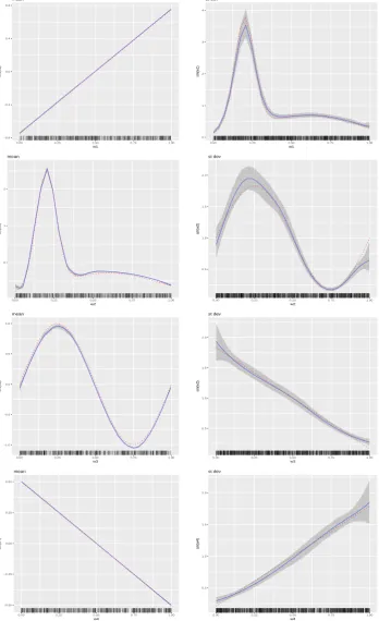
We conclude this section by presenting plots of the four terms in the mean and variance models. The plots are presented in Figure5. We provide a few details on how theplotmethod works in the presence of multiple terms, and how the comparison between true and estimated effects is made. Starting with the mean function, to create the relevant plots, that appear on the left panels of Figure5, theplotmethod considers only the part of the mean functionµ(u)that is related to the chosenterm

while leaving all other terms out. For instance, in the code below we chooseterm = "sm(u1)"and hence we plot the posterior mean and a posterior credible interval for∑16j=1β_1jφ_1j(u₁), where the

interceptβ0is left out by optionintercept = FALSE. Further, comparison is made with a centered version of the true curve, represented by the dashed (red color) line and obtained by the first three lines of code below.

> x1 <- seq(0, 1, length.out = 30) > y1 <- mu1(x1)

> y1 <- y1 - mean(y1)

> PlotOptions <- list(geom_line(aes_string(x = x1, y = y1),

+ col = 2, alpha = 0.5, lty = 2))

> plot(x = m3, model = "mean", term = "sm(w1)", plotOptions = PlotOptions, + intercept = FALSE, centreEffects = FALSE, quantiles = c(0.005, 1 - 0.005))

The plots of the four standard deviation terms are shown in the right panels of Figure5. Again, these are created by considering only the part of the model forσ(u)that is related to the chosenterm.

For instance, below we chooseterm = "sm(u1)". Hence, in this case the plot will present the posterior mean and a posterior credible interval for exp{∑16j=1α1jφ1j(u1)/2}, where the interceptα0is left out by optionintercept = FALSE. OptioncentreEffects = TRUEscales the posterior realizations of exp{∑16j=1α_1jφ_1j(u₁)/2}before plotting them, where the scaling is done in such a way that the realized

function has mean one over the range of the predictor. Further, the comparison is made with a scaled version of the true curve, where again the scaling is done to achieve mean one. This is shown below and it is in the spirit ofChan et al.(2006) who discuss the differences between the data generating mechanism and the fitted model.

> y1 <- stdev1(x1) / mean(stdev1(x1))

> PlotOptions <- list(geom_line(aes_string(x = x1, y = y1),

+ col = 2, alpha = 0.5, lty = 2))

> plot(x = m3, model = "stdev", term = "sm(w1)", plotOptions = PlotOptions, + intercept = FALSE, centreEffects = TRUE, quantiles = c(0.025, 1 - 0.025))

Data analyses

In this section we present four empirical applications.

Wage and age

−0.8 −0.4 0.0 0.4 0.8

0.00 0.25 0.50 0.75 1.00

w1

sm(w1)

mean

0 1 2 3 4

0.00 0.25 0.50 0.75 1.00

w1

sm(w1)

st dev

0 1 2

0.00 0.25 0.50 0.75 1.00

w2

sm(w2)

mean

0.5 1.0 1.5 2.0

0.00 0.25 0.50 0.75 1.00

w2

sm(w2)

st dev

−1.0 −0.5 0.0 0.5 1.0

0.00 0.25 0.50 0.75 1.00

w3

sm(w3)

mean

0.5 1.0 1.5 2.0

0.00 0.25 0.50 0.75 1.00

w3

sm(w3)

st dev

−0.50 −0.25 0.00 0.25 0.50

0.00 0.25 0.50 0.75 1.00

w4

sm(w4)

mean

0.5 1.0 1.5 2.0

0.00 0.25 0.50 0.75 1.00

w4

sm(w4)

st dev

Figure 5:Multiple covariate simulation study results. The column on the left-hand side presents the

● ● ● ● ● ● ● ● ● ● ● ● ● ● ● ● ● ● ● ● ● ● ● ● ● ● ● ● ● ● ● ● ● ● ● ● ● ● ● ● ● ● ● ● ● ● ● ● ● ● ● ● ● ● ● ● ● ● ● ● ● ● ● ● ● ● ● ● ● ● ● ● ● ● ● ● ● ● ● ● ● ● ● ● ● ● ● ● ● ● ● ● ● ● ● ● ● ● ●● ● ● ● ● ● ● ● ● ● ● ● ● ● ● ● ● ● ● ● ● ● ● ● ● ● ● ● ● ● ● ● ● ● ● ● ● ● ● ● ● ● ● ● ● ● ● ● ● ● ● ● ● ● ● ●● ● ● ● ● ● ● ● ● ● ● ● ● ● ● ● ● ● ● ● ● ● ● ● ● ● ● ● ● ● ● ● ● ● ● ● ● ● ● ● ● ● ● ● ● ● ● ● ● ● 11 12 13 14 15

0.00 0.25 0.50 0.75 1.00

nage sm(nage) mean 0.3 0.6 0.9

0.00 0.25 0.50 0.75 1.00

nage

sm(nage)

st dev

(a) (b)

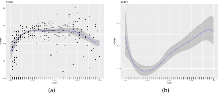
Figure 6:Results from the data analysis on the relationship between age and the logarithm of wage.

Panel (a) shows the posterior mean, an 80% credible interval of the mean function, and the observed data-points. Panel (b) shows the posterior mean and an 80% credible interval of the standard deviation function.

age. The dataset comes from the 1971 Census of Canada Public Use Sample Tapes and the sampling units it involves are males of common education. Hence, the investigation of the relationship between age and the logarithm of wage is carried out controlling for the two potentially important covariates education and gender.

We utilize the following R code to specify flexible models for the mean and variance functions, and to obtain 5, 000 posterior samples, after a burn-in period of 25, 000 samples and a thinning period of 5.

> data(cps71) > DIR <- getwd()

> model <- logwage ~ sm(age, k = 30, bs = "rd") | sm(age, k = 30, bs = "rd") > m4 <- mvrm(formula = model, data = cps71, sweeps = 50000,

+ burn = 25000, thin = 5, seed = 1, StorageDir = DIR)

After checking convergence, we use the following code to create the plots that appear in Figure6.

> wagePlotOptions <- list(geom_point(data = cps71, aes(x = age, y = logwage))) > plot(x = m4, model = "mean", term = "sm(age)", plotOptions = wagePlotOptions) > plot(x = m4, model = "stdev", term = "sm(age)")

Figure6(a) shows the posterior mean and an 80% credible interval for the mean function and it suggests a quadratic relationship betweenageandlogwage. Figure6(b) shows the posterior mean and an 80% credible interval for the standard deviation function. It suggest a complex relationship between

ageand the variability inlogwage. The relationship suggested by Figure6(b) is also suggested by the spread of the data-points around the estimated mean in Figure6(a). At ages around 20 years the variability inlogwageis high. It then reduces until about age 30, to start increasing again until about age 45. From age 45 to 60 it remains stable but high, while for ages above 60, Figure6(b) suggests further increase in the variability, but the wide credible interval suggests high uncertainty over this age range.

Wage and multiple covariates

In the second empirical application, we analyse a dataset fromWooldridge(2008) that is also available in the R packagenp. The response variable here is the logarithm of the individual’s hourly wage (lwage) while the covariates include the years of education (educ), the years of experience (exper), the years with the current employer (tenure), the individual’s gender (named asfemalewithin the dataset, with levelsFemaleandMale), and marital status (named asmarriedwith levelsMarriedand

Notmarried). The dataset consists ofn=526 independent observations. We analyse the first three covariates as continuous and the last two as discrete.

As the variance function is modeled in terms of an exponential, see (1), to avoid potential numerical problems, we transform the three continuous variables to have range in the interval[0, 1], using

> data(wage1)

> wage1$nexper <- wage1$exper / max(wage1$exper) > wage1$neduc <- wage1$educ / max(wage1$educ)

We choose to fit the following mean and variance models to the data

µi=β0+β1marriedi+f1(ntenurei) +f2(neduci) +f3(nexperi,femalei), log(σ_i2) =α0+f4(nexperi).

We note that, as it turns out, an interaction between variablesnexperandfemaleis not necessary for the current data analysis. However, we choose to add this term in the mean model in order to illustrate how interaction terms can be specified. We illustrate further options below.

> knots1 <- seq(min(wage1$nexper), max(wage1$nexper), length.out = 30) > knots2 <- c(0, 1)

> knotsD <- expand.grid(knots1, knots2)

> model <- lwage ~ fmarried + sm(ntenure) + sm(neduc, knots=data.frame(knots = + seq(min(wage1$neduc), max(wage1$neduc), length.out = 15))) +

+ sm(nexper, ffemale, knots = knotsD) | sm(nexper, knots=data.frame(knots = + seq(min(wage1$nexper), max(wage1$nexper), length.out=15)))

The first three lines of the R code above specify the matrix of (potential) knots to be used for represent-ingf3(nexper,female). Knots may be left unspecified, in which case the defaults in functionsmwill be used. Furthermore, in the specification of the mean model we usesm(ntenure). By this, we chose to representf1utilizing the default 10 knots and the radial basis functions. Further, the specification of f2in the mean model illustrates how users can specify their own knots for univariate functions. In the current example, we select 15 knots uniformly spread over the range ofneduc. Fifteen knots are also used to representf4within the variance model.

The following code is used to obtain samples from the posteriors of the model parameters.

> DIR <- getwd()

> m5 <- mvrm(formula = model, data = wage1, sweeps = 100000, + burn = 25000, thin = 5, seed = 1, StorageDir = DIR))

After summarizing results and checking convergence, we create plots of posterior means, along with 95% credible intervals, for functionsf1, . . . ,f4. These are displayed in Figure7. As it turns out, variablemarrieddoes not have an effect on the mean oflwage. For this reason, we do not provide further results on the posterior of the coefficient of covariatemarried,β1. However, in the code below we show how graphical summaries onβ1can be obtained, if needed.

> PlotOptionsT <- list(geom_point(data = wage1, aes(x = ntenure, y = lwage))) > plot(x = m5, model = "mean", term="sm(ntenure)", quantiles = c(0.025, 0.975), + plotOptions = PlotOptionsT)

> PlotOptionsEdu <- list(geom_point(data = wage1, aes(x = neduc, y = lwage))) > plot(x = m5, model = "mean", term = "sm(neduc)", quantiles = c(0.025, 0.975), + plotOptions = PlotOptionsEdu)

> pchs <- as.numeric(wage1$female)

> pchs[pchs == 1] <- 17; pchs[pchs == 2] <- 19 > cols <- as.numeric(wage1$female)

> cols[cols == 2] <- 3; cols[cols == 1] <- 2

> PlotOptionsE <- list(geom_point(data = wage1, aes(x = nexper, y = lwage), + col = cols, pch = pchs, group = wage1$female))

> plot(x = m5, model = "mean", term="sm(nexper,female)", quantiles = c(0.025, 0.975), + plotOptions = PlotOptionsE)

> plot(x = m5, model = "stdev", term = "sm(nexper)", quantiles = c(0.025, 0.975)) > PlotOptionsF <- list(geom_boxplot(fill = 2, color = 1))

> plot(x = m5, model = "mean", term = "married", quantiles = c(0.025, 0.975), + plotOptions = PlotOptionsF)

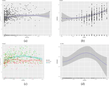
Figure7, panels (a) and (b) show the posterior means and 95% credible intervals forf1(ntenure)

and f2(neduc). It can be seen that expected wages increase with tenure and education, although there is high uncertainty over a large part of the range of both covariates. Panel (c) displays the posterior mean and a 95% credible interval for f3. We can see that although the forms of the two functions are similar, (i.e. the interaction term is not needed), males have higher expected wages than females. Lastly, panel (d) displays posterior summaries of the standard deviation function,σi=σexp(f4/2). It

● ● ● ● ● ● ● ● ● ● ● ● ● ● ● ● ● ● ● ● ● ● ● ● ● ● ● ● ● ● ● ● ● ● ● ● ● ● ● ● ● ● ● ● ● ● ● ● ● ● ● ● ● ● ● ●● ● ● ● ● ● ● ● ● ● ● ● ● ● ● ● ● ● ● ● ● ● ● ● ● ● ● ● ● ● ● ● ● ● ● ● ● ● ● ● ● ● ● ● ● ● ● ● ● ● ● ● ● ● ● ● ● ● ● ● ●●● ● ● ● ● ● ● ● ● ● ● ● ● ● ● ● ● ● ● ● ● ● ● ● ● ● ● ● ● ● ● ● ● ● ● ● ● ● ● ● ● ● ● ● ● ● ● ● ● ● ● ● ● ● ● ● ● ● ● ● ● ● ● ● ● ● ● ● ● ● ● ● ● ● ● ● ● ● ● ● ● ● ● ● ● ● ● ● ● ● ● ● ● ● ● ● ● ● ● ● ● ● ● ● ● ● ● ● ● ● ● ● ● ● ● ● ● ● ● ● ● ● ● ● ● ● ● ● ● ● ● ● ● ● ● ● ● ● ● ● ● ● ● ● ● ● ● ● ● ● ● ● ● ● ● ● ● ● ● ● ● ● ● ● ● ● ● ● ● ● ● ● ● ● ● ● ● ● ● ● ● ● ● ● ● ● ● ● ● ● ● ● ● ● ● ● ● ● ● ● ● ● ● ● ● ● ● ● ● ● ● ● ● ● ● ● ● ● ● ● ● ● ● ● ● ● ● ● ● ● ● ● ● ● ● ● ● ● ● ● ● ● ● ● ● ● ● ● ● ● ● ● ● ● ● ● ● ● ● ● ● ● ● ● ● ● ● ● ● ● ● ● ● ● ● ● ● ● ● ● ● ● ● ● ● ● ● ● ● ● ● ● ● ● ● ● ● ● ● ● ● ● ● ● ● ● ● ● ● ● ● ● ● ● ● ● ● ● ● ● ● ● ● ● ● ● ● ● ● ● ● ● ● ● ● ● ● ● ● ● ● ● ● ● ● ● ● ● ● ● ● ● ● ● ● ● ● ● ● ● ● ● ● ● ● ● ● ● ● ● ● ● ● ● ● ● ● ● ● ● ● ● ● ● ● ● ● ● ● ● ● ● ● ● ● ● ● ● ● ● ● ● ● ● ● ● ● ● 0 1 2 3

0.00 0.25 0.50 0.75 1.00

ntenure sm(nten ure) mean ● ● ● ● ● ● ● ● ● ● ● ● ● ● ● ● ● ● ● ● ● ● ● ● ● ● ● ● ● ● ● ● ● ● ● ● ● ● ● ● ● ● ● ● ● ● ● ● ● ● ● ● ● ● ● ● ● ● ● ● ● ● ● ● ● ● ● ● ● ● ● ● ● ● ● ● ● ● ● ● ● ● ● ● ● ● ● ● ● ● ● ● ● ● ● ● ● ● ● ● ● ● ● ● ● ● ● ● ● ● ● ● ● ● ● ● ● ● ● ● ● ● ● ● ● ● ● ● ● ● ● ● ● ● ● ● ● ● ● ● ● ● ● ● ● ● ● ● ● ● ● ● ● ● ● ● ● ● ● ● ● ● ● ● ● ● ● ● ● ● ● ● ● ● ● ● ● ● ● ● ● ● ● ● ● ● ● ● ● ● ● ● ● ● ● ● ● ● ● ● ● ● ● ● ● ● ● ● ● ● ● ● ● ● ● ● ● ● ● ● ● ● ● ● ● ● ● ● ● ● ● ● ● ● ● ● ● ● ● ● ● ● ● ● ● ● ● ● ● ● ● ● ● ● ● ● ● ● ● ● ● ● ● ● ● ● ● ● ● ● ● ● ● ● ● ● ● ● ● ● ● ● ● ● ● ● ● ● ● ● ● ● ● ● ● ● ● ● ● ● ● ● ● ● ● ● ● ● ● ● ● ● ● ● ● ● ● ● ● ● ● ● ● ● ● ● ● ● ● ● ● ● ● ● ● ● ● ● ● ● ● ● ● ● ● ● ● ● ● ● ● ● ● ● ● ● ● ● ● ● ● ● ● ● ● ● ● ● ● ● ● ● ● ● ● ● ● ● ● ● ● ● ● ● ● ● ● ● ● ● ● ● ● ● ● ● ● ● ● ● ● ● ● ● ● ● ● ● ● ● ● ● ● ● ● ● ● ● ● ● ● ● ● ● ● ● ● ● ● ● ● ● ● ● ● ● ● ● ● ● ● ● ● ● ● ● ● ● ● ● ● ● ● ● ● ● ● ● ● ● ● ● ● ● ● ● ● ● ● ● ● ● ● ● ● ● ● ● ● ● ● ● ● ● ● ● ● ● ● ● ● ● ● ● ● ● ● ● ● ● ● ● ● ● ● ● ● ● ● ● ● ● ● ● ● ● ● ● ● ● ● ● ● ● ● ● 0 1 2 3

0.00 0.25 0.50 0.75 1.00

neduc sm(neduc) mean (a) (b) ● ● ● ● ● ● ● ● ● ● ● ● ● ● ● ● ● ● ● ● ● ● ● ● ● ● ● ● ● ● ● ● ● ● ● ● ● ● ● ● ● ● ● ● ● ● ● ● ● ● ● ● ● ● ● ● ● ● ● ● ● ● ● ● ● ● ● ● ● ● ● ● ● ● ● ● ● ● ● ● ● ● ● ● ● ● ● ● ● ● ● ● ● ● ● ● ● ● ● ● ● ● ● ● ● ● ● ● ● ● ● ● ● ● ● ● ● ● ● ● ● ● ● ● ● ● ● ● ● ● ● ● ● ● ● ● ● ● ● ● ● ● ● ● ● ● ● ● ● ● ● ● ● ●● ● ● ● ● ● ● ● ● ● ● ● ● ● ● ● ● ● ● ● ● ● ● ● ● ● ● ● ● ● ● ● ● ● ● ● ● ● ● ● ● ● ● ● ● ● ● ● ● ● ● ● ● ● ● ● ● ● ● ● ● ● ● ● ● ● ● ● ● ● ● ● ● ● ● ● ● ● ● ● ● ● ● ● ● ● ● ● ● ● ● ● ● ● ● ● ● ● ● ● ● ● ● ● ● ● ● ● ● ● ● ● ● ● ● ● ● ● ● ● 0 1 2 3

0.00 0.25 0.50 0.75 1.00

nexper sm(ne xper ,ff emale) ffemale Female Male mean 0.2 0.3 0.4 0.5

0.00 0.25 0.50 0.75 1.00

nexper

sm(ne

xper)

st dev

(c) (d)

Figure 7: Results from the data analysis on the relationship between covariates gender, marital

status, experience, education, and tenure, and response variable logarithm of hourly wage. Posterior means and 95% credible intervals for (a) f1(ntenure), (b)f2(neduc), (c)f3(nexper,female), and (d) the standard deviation functionσi=σexp[f4(nexper)/2].

Lastly, we show how to obtain predictions and credible intervals for the levels"Married"and

"Notmarried"of variablefmariedand the levels"Female"and"Male"of variablefffemale, with variablesntenure,nedc, andnexperfixed at their mid-range.

> p1 <- predict(m5, newdata = data.frame(fmarried = rep(c("Married", "Notmarried"), 2), + ntenure = rep(0.5, 4), neduc = rep(0.5, 4), nexper = rep(0.5, 4),

+ ffemale = rep(c("Female", "Male"), each = 2)), interval = "credible")

> p1

fit lwr upr

1 1.321802 1.119508 1.506574 2 1.320400 1.119000 1.505272 3 1.913341 1.794035 2.036255 4 1.911939 1.791578 2.034832

The predictions are suggestive of no “marriage” effect and of “gender” effect.

Brain activity

Here we analyse brain activity level data obtained by functional magnetic resonance imaging. The dataset is available in packagegamair(Wood,2006) and it was previously analysed byLandau et al. (2003). We are interested in three of the columns in the dataset. These are the response variable,medFPQ, which is calculated as the median over three measurements of “Fundamental Power Quotient” and the two covariates,XandY, which show the location of each voxel.

The following R code loads the relevant data frame, removes two outliers and transforms the response variable, as was suggested byWood(2006). In addition, it plots the brain activity data using functionlevelplotfrom the packagelattice(Sarkar,2008).

> data(brain)

Y

X

50 60 70 80

10 20 30 40 50

0.5 1.0 1.5 2.0

Y

X

50 60 70 80

10 20 30 40 50

0.8 1.0 1.2 1.4 1.6 1.8 2.0

(a) (b)

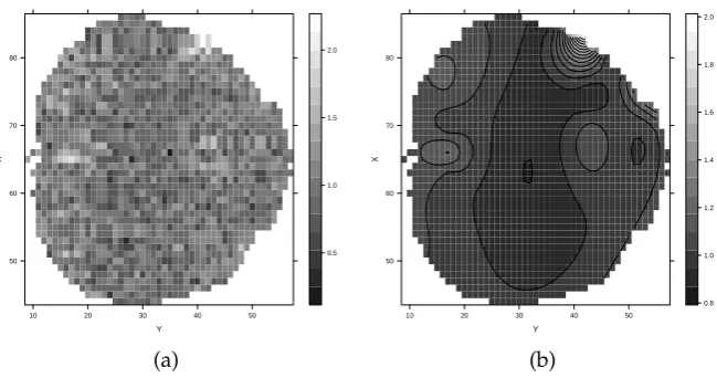
Figure 8:Results from the brain activity level data analysis. Panel (a) shows the observed data and

panel (b) the model-based smooth surface.

> levelplot(medFPQ ~ Y * X, data = brain, xlab = "Y", ylab = "X", + col.regions = gray(10 : 100 / 100))

The plot of the observed data is shown in Figure8, panel (a). Its distinctive feature is the noise level, which makes it difficult to decipher any latent pattern. Hence, the goal of the current data analysis is to obtain a smooth surface of brain activity level from the noisy data. It was argued by Wood(2006) that for achieving this goal a spatial error term is not needed in the model. Thus, we analyse the brain activity level data using a model of the form

medFPQ_iind∼ N(µi,σ2), whereµi=β0+ 10

∑

10

∑

βj1,j2φ1j1,j2(Xi,Yi),i=1, . . . ,n,

wheren=1565 is the number of voxels.

The R code that fits the above model is

> Model <- medFPQ ~ sm(Y, X, k = 10, bs = "rd") | 1

> m6 <- mvrm(formula = Model, data = brain, sweeps = 50000, burn = 20000, thin = 2, + seed = 1, StorageDir = DIR)

From the fitted model we obtain a smooth brain activity level surface using functionpredict. The function estimates the average activity at each voxel of the brain. Further, we plot the estimated surface using functionlevelplot.

> p1 <- predict(m6)

> levelplot(p1[, 1] ~ Y * X, data = brain , xlab = "Y", ylab = "X", + col.regions = gray(10 : 100 / 100), contour = TRUE)

Results are shown in Figure8, panel(b). The smooth surface makes it much easier to see and understand which parts of the brain have higher activity.

Cars

In the fourth and final application we use the functionmvrmto identify the best subset of predictors in a regression setting. Usually stepwise model selection is performed, using functionsstepfrom base R andstepAICfrom theMASSpackage. Here we show howmvrmcan be used as an alternative to those two functions. The data frame that we applymvrmon ismtcars, where the response variable ismpg

and the explanatory variables that we consider aredisp,hp,wt, andqsec. The code below loads the data frame, specifies the model and obtains samples from the posteriors of the model parameters.

> data(mtcars)

> Model <- mpg ~ disp + hp + wt + qsec | 1