Private Debt with Pervasive Default Risk

Munich Personal RePEc Archive

Private Debt with Pervasive Default Risk

Gao, Xiang

Iowa State University

1 September 2009

Online at

https://mpra.ub.uni-muenchen.de/18379/

Private Debt with Pervasive Default Risk

Xiang Gao

Iowa State University

This Draft: November 2009

Abstract

This paper studies the e¤ects of private debts on risk sharing and welfare, in which I assume individual

residents have access to both international and domestic capital markets. Like Jeske (2006), I make the

assumption that domestic residents cannot commit to repay their debts across border. The previous

literature assumes contracts are perfectly enforceable within border, and hence the marginal rate of

substitution must be equal among all residents in any one country. The novel feature in this model

is to bring limited commitment into debt contracts signed between domestic residents. The pervasive

risk of repudiation creates di¤erent domestic asset pricing rules for countries that are constrained in

international …nancial market. Constrained country’s domestic interest rate is equal to the reciprocal

of the lowest marginal rate of substitution within that country. However, non-constrained countries

still have equalized marginal rate of substitution which determines the international interest rate. A

wider gap between domestic and international …nancing cost emerges in this model and leads to harsher

punishment for international debt defaulters. Although limited domestic risk sharing hinders aggregate

welfare reaching an even higher standard, it has no negative e¤ect on the original level in Jeske’s setup. As

a result, my model allows more international risk sharing and higher welfare. I show how this improvement

depends on the interaction between preventing within and across border default in equilibrium. I also

explore the role of endogenous borrowing constraints, international borrowing by using other domestic

residents as intermediaries and the speci…cation of deviation penalty.

Keywords: Default risk, private debt, limited commitment.

JEL Classification: F34, F41.

I am thankful to John Schroeter, Rajesh Singh for helpful comments and suggestions. All remaining errors are mine.

Address for correspondence: Department of Economics, 477 Heady Hall, Iowa State University, Ames IA 50011. E-mail:

1

Introduction

In the presence of limited commitment, regardless of complete …nancial markets, international loans are

available only to the extent that their repayments can be enforced by the threat of reversion to autarky.

Frictions of this kind result in limited risk sharing between countries across the world. The size of risk

sharing is determined by the speci…cation of the outside option. Jeske (2006) predicts that a centralized

arrangement, where only government borrows internationally and redistributes domestically, allows more

international risk sharing and higher aggregate welfare than a decentralized arrangement, where individual

residents have access to capital markets. An intuitive proof is as follow. One can think of the decentralized

arrangement as a centralized setup only this imaginary government assumes that it can ignore the resource

constraint in autarky after default and instead keep borrowing at domestic interest rate just like residents,

which is a better outside option than pure autarky in the original centralized arrangement. Higher

post-default value leads to tighter participation constraint in international …nancial market and accordingly smaller

capital ‡ow. A crucial assumption in this proof is that domestic debts are perfectly enforceable. For this

very reason, the decentralized arrangement is equivalent to an corresponding imaginary planner’s problem,

in which the marginal rate of substitution (MRS, from now on) is equalized across all residents within any

country.

In this paper, I add limited commitment problem in debt contracts signed between domestic residents.

This revision introduces a new way of deviation from risk sharing agreement: domestic debt default. The

penalty for domestic debt defaulters is harsher than international debt defaulters. While international debt

defaulters are excluded from international …nancial market but retain access to domestic …nancial market,

domestic debt defaulters are prohibited to participate in all …nancial markets. This assumption of some

discrimination against foreign creditors seems to me more realistic than the previous one of in…nite

dis-crimination in which domestic creditors are fully protected. This paper shows that limited commitment

of domestic debts has opposite e¤ects on country’s aggregate welfare after globalization. Pervasive risk of

default may hamper domestic exchange and worsen welfare, whereas it can raise the volume of international

capital ‡ow thus improve welfare. The reason for the latter statement is as follow. Thanks to participation

constraints in domestic …nancial market, international debt defaulters now confront more severe punishment

than before. After a default, the channel of using other non-defaulted domestic residents as intermediaries

to access international …nancial market is restricted. In contrast, international debt defaulters in Jeske’s

ques-tion then is which e¤ect dominates. I prove that when residents are heterogeneous and there exist some

residents who are sometimes on the edge of reneging on domestic debt, the positive e¤ect enables these

residents to enjoy welfare gains from an increment in foreign capital ‡ow while the welfare levels for others

stay una¤ected. Although the negative e¤ect hinders aggregate welfare reaching an even higher standard

when comparing with a centralized distribution mechanism, it is not functioning as by reference to Jeske’s

decentralized arrangement. Therefore, more international risk sharing and higher (at least the same if there

are no indi¤erent residents) aggregate welfare can be supported in my amended model when comparing with

Jeske’s decentralized arrangement. The policy implication is that perfect domestic risk sharing and in…nite

discrimination against foreign creditors together lower the level of international risk sharing if pervasive risk

of default is a fact of life. There is a rationale for government in decentralized countries to exchange perfect

domestic enforcement for better international connections.

Now that aggregate welfare has been improved by not enforcing domestic debt contracts, does

govern-ments still want to control private capital and carry out the centralized arrangement? The answer depends

on the trade-o¤ that centralization wins by gains from domestic exchange but may lose by few gains from

international exchange. In a numerical example, I show that capital control is always the best disregarding

domestic limited commitment if the endowment structure is such that international income ‡uctuation is

large relative to domestic income ‡uctuation.

The novel commitment problem within border also overturns the domestic bond pricing rule for countries

that are participation constrained in equilibrium. In closed economy models with heterogeneous residents,

domestic interest rate is determined by the highest MRS possible in that economy to ensure repayment.1 _In

open economy models with perfect domestic enforcement, international interest rate is determined by the

highest MRS in all countries across the world, whereas domestic interest rate is determined by the equalized

MRS within any country.2 _{In this model, international interest rate is, as usual, determined by highest}

MRS, however, domestic interest rate is equalized to the reciprocal of the lowest MRS among all residents.

This result is consistent with the assumption that international debt defaulters are penalized harsher in my

model. When international debt defaulters come down to seeking help in domestic …nancial market, they

face a wider gap between domestic and international …nancing cost since domestic bond price is lower than

ever. This cruel situation raises international borrowing quota for all residents and pays o¤ by higher welfare

1_{Bond price is negatively related to corresponding interest rate. When price is determined by the highest MRS, interest rate}

level.

Of critical importance in this strand of literature is the speci…cation of what defaulters may be entitled.

In the remainder of this section, I review several closely related work which try to relax the assumption of

compelet exclusion from future trading in early theories.3

A growing research body uses the assumption of partial exclusion, under which defaulters retain some

access to …nancial markets or have alternative ways to smooth consumption. International risk sharing

diminishes in size since life after default is less painful than it would be otherwise. Partial exclusion arises

if defaulters can reenter foreign capital market indirectly through intermediaries as in Jeske (2006). Wright

(2006) builds on Jeske’s model and argues that international borrowing subsidies can also lead to constrained

e¢cient allocations instead of Jeske’s radical way of centralization. Defaulters continuing to have access to

international savings may also cause partial exclusion. Bulow and Rogo¤ (1989) …rst use this idea and prove

that international borrowing cannot be supported in a small open economy that takes the international

interest rate as given (partial equilibrium). Hellwig and Lorenzoni (2007) carry their work further to a

multi-country (general equilibrium) setup in which they show that international risk sharing can exist with

low interest rate. Then Wright establishes an equivalence between the above two modeling methods if the

extra dimension of heterogeneity among residents in Jeske’s model is taken care of. Reduced penalty can be

due to other internal opportunities as well. For example, Kehoe and Perri (2002, 2004) study international

risk sharing in a real business cycle model under productivity shock, in which autarky value depends on the

quantity of capital the country has accumulated up to defaults. In their paper, defaulters can continue to

produce and consume capital inautarky, but they may not buy or sell capital and other …nancial assets to

foreigners.

Broner and Ventura (2009) assume that countries cannot discriminate against foreign creditors. Thus,

international risk sharing is obtained even in the absence of international debt default penalties. Unlike my

model in which residents make default decisions, in their setup government endogenously chooses whether

to enforce all debt contracts or none. They show that decrease in trade barriers in goods market facilitates

international trade and raises the costs of enforcement. As a result, globalization might hamper domestic

trade and lower aggregate welfare. In this paper, government can identify the citizenship but still chooses

to enforce none because more international risk sharing can be supported.

3_{See, for example, Kehoe and Levine (1993), Kocherlakota (1996), Alvarez and Jermann (2000) and Kehoe and Perri (2002,}

The remainder of the paper is organized as follows. In section 2, I present the model of private

in-ternational lending and borrowing with limited commitment problem within and across border and derive

equilibrium results. Section 3 compares aggregate welfare level in di¤erent setups, thus generates some policy

implications. Section 4 introduces a crude numerical example which illustrates the essence of this paper.

Section 5 concludes and …nally a technical appendix contains all proofs.

2

The Model

The model considers a world that consists of a …nite number of countries denoted asm2 f1;2; :::; Mgand each

countrymis populated byNtypes of residents with a continuum of them in each typen2 f1;2; :::; Ng:4

Res-idents live forever so that time is in…nite and discrete, denoted byt= 0;1;2; :::;1:Information about current

and future endowments is indexed by the state t2 :History is summarized in t f 0; 1; 2; :::; tg 2 t

with 0given. Transition probability from history tto next period’s state t+1is known as ( t+1j t)with

t _{given. (} t_{)is the unconditional probability of observing history} t_{and (} r_j t_{)is the probability of}

ob-serving history r conditional on having been in t:There is only one non-storable consumption good which

can be exchanged within and across border. I denote byem

n( t)the endowment of typenin countrymafter history tand bycm_n( t)the corresponding consumption. There are M domestic bonds for each countrym

and only one international bond traded across the world. Let bm

n( t; t+1)and fnm( t; t+1)respectively be the amounts of domestic and foreign state-contingent securities held by agents of typenliving in countrym;

which are purchased at t and for payment next period in state t+1;pm( t; t+1)and q( t; t+1)are their

respective prices.

For allnandm, I use 2(0;1)as the discount factor and denote byU( )the period utility function which

is strictly increasing, strictly concave, and twice continuously di¤erentiable. Typenresidents in country m

have preferences

1

X

r=t

r t X

r_j t

( rj t)U(cm

n( r));

4_{Unlike Jeske, I assume that in any countrymthe mass of typenresidents} m

n is normalized to1for alln2 f1;2; :::; Ng:

Note that in Jeske’s model one’s endowment only depends on type. Although living in di¤erent countries, same types receive

the same endowment each period. As a result, having m

n = 1for allnandmin Jeske would imply that countries are identical

ex-ante, thus there may not be any role for international capital ‡ow. However, in this paper one’s endowment vary upon both

type and country, which will be clear after I introduce history and endowment structure. Assuming m

n = 1simpli…es notation,

after twitht2[0;1):

I take the existence of limited commitment problem as a fact of life. In particular, debt contracts

between any two parties are not enforced. Previous theories have instead assumed that debt contracts

between domestic residents and foreigners are not enforced while all domestic payments are perfectly enforced.

Border still matters here because default within border leads to di¤erent penalty from default across border.

International debt defaulters can still trade internationally indirectly, through borrowing from other

non-defaulted domestic residents in the same country. I refer this situation as resident’s international autarky

henceforth. However, domestic debt defaulters would be denied from all …nancial markets, which I call

resident’s autarky hereafter.

Despite the fact whether residents have defaulted on international debt or not, the continuation value for

typenresidents in countrymwho renege on domestic debt at ris

Am_n( r)

1

X

s=r

s r X

s_jr

( sj r)U(em_n( s)): (RA)

De…nition 1 Typenresidents in countrymlive inresident’s autarky after any history r if their period

consumptioncm;A

n (

s_{) =}

em

n(

s_{)for all histories} s_with

s2[r;1):

Since all residents are small relative to the market, individual defaulter on international debt does so at

t _{by assuming that the sequence of all future domestic bond pricesf}

pm₍ r

; r+1)g_r2[t;1)stays unchanged.

Consider type n residents in country m who renege on international debt alone at t, their continuation

value in resident’s international autarky can be represented as

V_nm( t; bm_n( t)) max

fcm

n(r);bmn(r; r+1)gr2[t;1)

1

X

r=t

r t X

r_j t

( rj t)U(cm_n( r)); (RIA)

subject to the budget constraint

em

n( r) +bmn( r)>cmn( r) +

X

r+1

pm₍ r_;

r+1)bmn( r; r+1); (1)

the participation constraint in domestic …nancial markets

1

X

s=r

s r X

s_jr

( sj r)U(cm_n( s))>Am_n( r); (2)

the no-Ponzi condition

bm_n( r_;

r+1)> B;

with

for all histories rand states( r; r+1)withr2[t;1): bmn( t)denotes the domestic bond holdings residents

inherit when entering periodt: B >0is large enough such that no-Ponzi conditions never bind in equilibrium,

which ensures compactness of the budget set. For the problem to be interesting, I assume for somen; mand

t _{there exist future histories} r _{at which domestic participation constraints (2) are binding.}

Unlike Jeske’s model, in which domestic debt default is not allowed in nature though it might be a better

choice in some future histories r if

1

X

s=r

s r X

s_j r

( sj r)U(cm_n( s))< Am_n( r)withr > t;

this model prevents domestic debt defaults at all future histories r withr2[t;1) by a set of constraints

(2).

De…nition 2 Given a price sequencefpm₍ r_;

r+1); q( r; r+1)gr2[t;1) and domestic bond holdings bmn( t);

type n residents in country m live in resident’s international autarky after any history t if their

consumption allocation fcm;D

n ( r)gr2[t;1) solves resident’s international autarky problem (RIA).

Up to now, I have de…ned the outside options for domestic debt defaulters in (RA) and international

debt defaulters in (RIA). We are ready to write down resident’s problem before any default. Residents

choose sequences for consumption and for both domestic and international bond holdings to maximize life

time preference

max

fcm

n( t);bmn( t;t+1);fnm( t;t+1)gt2[0;1)

1

X

t=0

tX

t

( t)U(cm_n( t)); (RP)

subject to the budget constraint

em_n( t) +bm_n( t) +f_nm( t)

> cm_n( t) +X

t+1

pm( t; t+1)bmn( t

; t+1) + X

t+1

q( t; t+1)fnm( t

; t+1); (3)

the participation constraint in international …nancial markets

1

X

r=t

r t X

r_j t

( rj t)U(cm

n( r))>Vnm( t; bmn( t)); (4)

the participation constraint in domestic …nancial markets

1

X

r=t

r tX

r_jt

( rj t)U(cm_n( r))>Am_n( t); (5)

the no-Ponzi conditions

with initial bond holdings

bm_n( 0); f_nm( 0)given

and bond price sequences

pm( t; t+1); q( t; t+1)given,

for all histories tand states t; t+1 witht2[0;1):No-Ponzi conditions again require B and F >0 to

be large enough to ensure that these two constraints never bind.

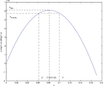
To solve the problem, notice that international participation constraint (4) implies the domestic

partici-pation constraint (5) for all twitht2[0;1):By de…nition,

V_nm( t_{; b}m

n( t))>Amn( t)for all t:

The reason is that problem (RA)’s consumption allocation cm;A

n ( r) _r2[t;1)is always a¤ordable and

individ-ual rational in problem (RIA). Intuitively, no one reneges on domestic debt before a default on international

debt in equilibrium. This is a direct result from the assumption of harsher penalty for domestic debt

de-faulters than international debt dede-faulters. Hence, constraint (5) is redundant in …nding optimal solutions as

can be seen in Figure 1. This cut simpli…es life since domestic enforcement problem will only a¤ect optimal

allocation indirectly through the utility level of resident’s international autarky, i.e.,Vm

n (

t

; bm

n(

t_{)). Rest of}

this section …rst de…nes, then characterizes the equilibrium results.

De…nition 3 A trade equilibrium is an allocation fcm

n(

t₎

; bm

n(

t

; t+1); fnm( t

; t+1)gt2[0;1) and a price

sequencefpm₍ t_;

t+1); q( t; t+1)gt2[0;1) such that each type solves resident’s problem (RP) given prices and

initial bond holdings, while resource feasibility

M X

m=1

N X

n=1

cm_n( t)

M X

m=1

N X

n=1

em_n( t);

domestic …nancial markets clearing condition

N X

n=1

bm_n( t; t+1) = 0; for allm;

and international …nancial market clearing condition

M X

m=1

N X

n=1

f_nm( t_;

t+1) = 0;

The Lagrangian of the resident’s problem (RP) is (drop the superscript and subscript for simplicity)

LRP =

1

X

t=0

tX

t

( t)U(c( t)) +

+ 1 X t=0 X t

( t_{) e(} t_{) +b(} t_{) +f(} t_{) c(} t₎

1

X

t=0

X

t

( t_{) p(} t_;

t+1)b( t; t+1) +q( t; t+1)f( t; t+1)

+ 1 X t=0 X t

( t₎ 2

4

1

X

s=t

s t X

s_j t

( s_j t_)U(c( s_{)) V(} t_{; b}m

n( t))

3

5;

where m

n(

t_{) and} m

n(

t_{) denote respectively the Lagrange multipliers on the budget constraint (3) and}

international participation constraint (4) if toccurs.

First order conditions are: with respect to c( t);

t ₍ t₎

U0(c( t)) ( t) +

t X

s=0

( s) t s X

t_j s

( tj s)U0(c( t)) = 0; (6)

with respect tob( t; t+1);

p( t_;

t+1) ( t) + ( t; t+1) ( t; t+1)

dV( t; t+1; b( t; t+1))

db( t; t+1)

= 0; (7)

and with respect tof( t; t+1);

q( t; t+1) ( t) + ( t; t+1) = 0: (8)

Rearrange (6) to get

( t) = r t ( t)U0(c( t))

2

41 +

t X

s=0

X

t_j s

( s) s (

t_j s₎

( t)

3

5: (9)

Before using (7), I went back and solved the post-default optimization problem (RIA) in order to get a closed

form of its envelope condition, dV( t;t+1;b( t;t+1))

db( t_;

t+1) .

To solve (RIA) with initial history t, …rst write down the Lagrangian.

LRIA =

1

X

r=t

r t X

r_j t

( rj t)U(c( r))

+

1

X

r=t

X

r_j t

( r)

2

4e( r) +b( r) c( r) X

r+1

p( r; r+1)b( r; r+1) 3

5

+

1

X

r=t

X

r_j t

( r)

2

4

1

X

s=r

s r X

s_j r

( sj r)U(c( s)) Am_n( r)

3

Let mn( r)and mn( r)be the multipliers on the budget constraint (1) and domestic participation constraint

(2) if r occurs. First order condition with respect toc( r)is

r t ₍ r_j t₎

U0(c( r)) ( r) +

r X

s=t

( s) r s X

r_js

( rj s)U0(c( r)) = 0:

Rewrite it to get

( r) = r t ( rj t)U0(c( r))

2

41 +

r X

s=t

X

r_js

( s) t s (

r_j s₎

( rj t)

3

5: (10)

Given initial domestic bond holdingsbm

n( t);envelope theorem yields

dV( t; b( t))

db( t₎ =

@LRIA

@b( t₎ = (

t₎

: (11)

Combine (10) and (11) together.

dV( t_{; b(} t₎₎

db( t) =

t t ₍ t_j t_)U0_(cD₍ t₎₎

2

41 +

t X

s=t

X

t_js

( s) t s (

t_j s₎

( tj t)

3

5

= 1 + ( t) U0(cD( t));

where cD( t)is the …rst element in the optimal consumption allocation cD( r) _r2[t;1) that solves (RIA)

with initial history t. Iterating dV(_dbt₍;bt(₎t)) one period forward generates

dV( t; t+1; b( t; t+1))

db( t; t+1)

= 1 + ( t; t+1) U0(cD( t; t+1)): (12)

Now continue with problem (RP). Substitute (12) into (7) and solve for the domestic bond price together

with (9).

p( t; t+1) =

( t; t+1) ( t; t+1)dV(

t_;

t+1;b( t;t+1))

db( t_;

t+1)

( t)

= (

t_;

t+1) ( t; t+1) 1 + ( t; t+1) U0(cD( t; t+1))

( t₎

= U

0_(c( t

; t+1))

U0_(c( t₎₎ ( t+1j

t₎1 +A2 1 + ( t; t+1) A1 1 +A3

; (13)

where

A1 = ( t; t+1) t 1

U0(cD₍ t

; t+1))

U0_(c( t_;

t+1))

1 ( t; t+1)

;

A2 =

t+1

X

s=0

X

t_; t+1js

( s) s (

t_;

t+1j s)

( t; t+1)

;

A3 =

t X

s=0

X

t_js

( s) s (

t_j s₎

Finally, solve for international bond price with (8) and (9).

q( t; t+1) =

( t; t+1)

( t)

= U

0_(c( t

; t+1))

U0_(c( t₎₎ ( t+1j

t₎1 +A2

1 +A3

: (14)

Most propositions in this section closely follow Jeske (2006) with slight change to accommodate the

enforcement problem within border. In country m; consider residents of some types n f1;2; :::; Ng for

whom m

n( t) > 0 with t 2 [0;1); i.e., they are internationally participation constrained at t in trade equilibrium. In contrast to the work by Jeske, these constrained types might be di¤erent from each other

because of domestic enforcement problem. Speci…cally, typenresidents fall into two categories: typenAand

nB with nA [nB = n: In resident’s international autarky, type nA with vmnA(

r_{) = 0 for all r 2 [t;1)}

are never domestically participation constrained while type nB with vmnB(

r₎

> 0 for some r 2 [t;1) are

sometimes domestically participation constrained at r:

Typen residents at the brink of default attain the same continuation value by staying with trade

equi-librium and reversing to resident’s international autarky. Proposition 1 states that typesnalso consume the

same amount of goods at every future history from t on irrespective of reneging on international debt.

Proposition 1 In trade equilibrium, if m

n(

t₎

>0 for somen; mand twitht2[0;1);thencm;D

n (

r_)and

cm

n( r)are identical for all rhappening with positive probability andr2[t;1);where cm;Dn ( r) _r2[t;1)and

fcm

n(

r_)g

r2[0;1) respectively denote the optimal consumption allocations in resident’s international autarky

problem (RIA) started at r and in resident’s problem (RP).

Proof. See Appendix A.1.

I get the same result above as in Jeske’s (2006) proposition 1, which has been extremely useful in

proving all following propositions. Proposition 2 states that, for any country and history, either every type

is internationally participation constrained or no type is, even if types are heterogeneous.

Proposition 2 For allmand( t; t+1)witht2[0;1);eitherq( t; t+1)> pm( t; t+1)and mn(

t

; t+1)>

0 for alln; orq( t; t+1) =pm( t; t+1)and mn( t; t+1) = 0 for alln:

Proof. See Appendix A.2.

All types in countrym must be participation constrained in international …nancial market at the same

time. Otherwise, it would be pro…table for non-constrained types to borrow internationally up to their

constraints and relend at a higher interest rate to constrained ones. No arbitrage in equilbrium allows us

result is again the same as Jeske’s (2006) proposition 4. Removing the assumption of perfectly enforceable

contracts within border, therfore, does not alter the basic characteristics of countries that are internationally

participation constrained in trade equilibrium. However, within the border of any constrained country,

domestic enforcement problem a¤ects the restrictions imposed on typenBwhen participating in international

…nancial market.

If typenBresidents from one internationally constrained country indeed choose to default on international

debt at tand instead live in resident’s international autarky thereafter, then they will again …nd themselves

indi¤erent between reneging on and repaying domestic debt at some future history r:Proposition 3 says that

typenB residents can neither borrow nor lend domestically beyond some constant domestic debt holdings

at t 1in trade equilibrium.

Proposition 3 In trade equilibrium, for some n; m and t with t 2 (0;1); if m

n( r) > 0 at r with

r2[t;1)in addition to m

n(

t₎

>0; then

bm

n( t) =B

m

n( t);

whereBm_n( t)is some constant determined by

1

X

s=r

s r X

s_j r

( sj r)U(cm;D_n ( s; t; Bm_n( t))) =Am_n( r):

Proof. See Appendix A.3.

when it comes to decide the domestic bond holdingsbm

nB(

t_)at t 1_;typen

B residents in internationally

constrained country must buy a speci…ed amountBm_nB( r_{)even if they want to borrow or lend more. This} observation is critical to prove the next two propositions. Meanwhile, typenAresidents in the same country

can freely choose their domestic bond holdings, but they do not want to deviate whenever the optimum is

arrivied.

In general, the international participation constraint (4) makes resident’s problem (RP) non-convex.

Proposition 4 justi…es the su¢ciency of …rst-order-condition approach for a maximum. A similar method

has been used in the proof of Jeske’s (2006) proposition 2. First of all, I de…ne an alternative maximization

problem with the same objective function and a convex constraint set that is a superset of the non-convex

constraint set in the original non-convex problem. Then I show that a solution to the original problem is

also a¤ordable and individually rational in the alternative convex problem. It turns out that both problems

have identical …rst order conditions, thus the same optimal solutions. Therefore, the …rst order conditions

Proposition 4 For alln andm;together with a transversality condition

lim

T!1

TX

T

U0(cm_n( T)) ( T)hbm_n( T) +f_nm( T)i= 0;

…rst order conditions (7), (8) and (9) are su¢cient to characterize the maximum of (RP).

Proof. See Appendix A.4.

Proposition 5 shows how domestic and international bond prices are determined in trade equilibrium.

The domestic bond pricing rule di¤ers from the one in Jeske’s (2006) proposition 3 since MRS’s across

di¤erent types in any internationally constrained country are no longer equalized in general.

Proposition 5 In trade equilibrium, for all n; mand t; t+1 witht2[0;1);

(I) the international bond price in the world is

q( t; t+1) = max

m=1;:::;M;n=1;:::;N

U0_(cm

n( t; t+1))

U0_(cm

n( t))

( t+1j t) ;

(II) the domestic bond price in country m2 f1;2; :::; Mg is

pm( t; t+1) = min

n=1;:::;N

U0_(cm

n( t; t+1))

U0_(cm

n(

t₎₎ ( t+1j t) ;

and …nally

(III) the relationship between international bond price and allM domestic bond prices is

q( t; t+1) = max

m=1;:::;M p

m₍ t

; t+1) :

Proof. See Appendix A.5.

In the …rst part, the international bond price is equal to the maximum MRS among allN types and across

allM countries. Intuitively, international interest rate has to be to the lowest so that repaying international

debt would not hurt debtors as much as living isolated from the world.

The second part says that the domestic bond price in m is equal to the minimum MRS among allN

types inm. This rule overturns the result from closed economy models in which price must be the highest to

guarantee the incentive of ful…lling debtor’s obligation. The reason is that domestic debt default can never

occur without an international debt default in this paper. In contrast to closed economy models, domestic

interest rate as a device to ensure repayment is no longer needed. Instead, domestic interest rate plays

Consider a country with m

n( t; t+1)>0 for example. When its residents are contemplating international debt default, they …nd themselves more miserable in resident’s international autarky since the domestic

interest rate is higher than the level they would have accepted. Country with m

n( t; t+1) = 0 is a special case in part two since the MRS’s are equalized among allN types in this unconstrained country. Moreover,

its domestic bond price must equal to the international bond price in order to rule out the possibilities

of arbitrage. All the above results combining together reveals the relationship between international and

domestic bond prices in the thrid part.

3

Welfare Analysis

In this section, I rank the aggregate welfare level in two scenarios for any country m2 f1;2; :::; Mg. The

…rst scenario is Jeske’s private international borrowing setup in which only debt contracts across border are

subject to the risk of repudiation. The second scenario is my decentralized model presented in section 2,

in which both within and across border contracts are not enforced. I can show that countrym’s aggregate

welfare in my model is higher than Jeske’s setup given some exogenous welfare-weighted index.

Recall Jeske (2001, 2006), after type nresidents in country m renege on international debt at t, their

value can be represented as

V_nm;J( t; bm_n( t)) max

fcm

n( r);bmn( r; r+1)gr2[t;1)

1

X

r=t

r tX

r_j t

( rj t)U(cm_n( r)); (RIAJ₎

subject to the budget constraint

em_n( r) +bm_n( r)>cm_n( r) +X

r+1

pm( r; r+1)bmn( r

; r+1);

the no-Ponzi condition

bm_n( r; r+1)> B;

with

bm_n( t)andpm( r; r+1)given,

for all histories r _{and all states(} r_;

r+1)withr2[t;1):

Again at date0before any default could happen, resident’s problem is to choose sequences for

consump-tion and for holdings of both domestic and internaconsump-tional bonds to maximize life time utility

max

fcm

n( t);bmn( t;t+1);fnm( t;t+1)gt2[0;1)

1

X

t=0

tX

t

subject to the budget constraint

em_n( t) +bm_n( t) +f_nm( t)

> cm_n( t) +X

t+1

pm( t; t+1)bmn( t

; t+1) + X

t+1

q( t; t+1)fnm( t

; t+1);

the participation constraint in international …nancial markets

1

X

r=t

r tX

r_jt

( rj t)U(cm_n( r))>V_nm;J( t; bm_n( t)); (15)

the no-Ponzi conditions

bm_n( t; t+1)> B; fnm( t; t+1)> F ;

with initial bond holdings

bm_n( 0); f_nm( 0)given

and bond price sequences

pm( t; t+1); q( t; t+1)given,

for all histories tand all states t; t+1 witht2[0;1):

For any m;all types in my model achieve higher or at least the same welfare level than in Jeske’s setup

above. One intuitive explanation is that type nB residents now confront with more severe penalty after

international debt default (lower continuation value in resident’s international autarky). Assume a small open

economym stops enforcing domestic contracts after a bad shock. TypenA’s optimization problem can still

be de…ned by (RPJ_{), thus their welfare level stays the same. However, typen}

B’s optimization problem shifts

from (RPJ_{) to (RP). Typesn}

B residents’ original optimal allocations in (RPJ) are both a¤ordable in (RP),

since bond prices determined by typenAstay unchanged, and individual rational in (RP), since international

participation constraints (4) are less tighter than (15) and the newly added domestic participation constraints

(5) are super‡uous. If there do exist type nB residents whose domestic participation constraints (2) bind

after some future histories in (RIA) when their country is internationally constrained after some present

histories in (RP), and if there are positive international capital in‡ows at these present histories in (RP),

then type nB residents after the shock can do strictly better by relaxing their international participation

constraints (4) at present histories in (RP). Adding up welfare levels of all types with exogenously given

weights assigned to each type, the country’s aggregate welfare is improved since typenA residents stay the

Proposition 6 Assume the welfare-weighted index is given by f'm

ng

N

n=1 with 'mn 2 R++ for all n in

any m. Let cm n

t

; bm

n(

t

; t+1); fnm( t

; t+1)

t2[0;1) solves resident’s problem (RP) in section 2 and

cm;J

n t ; bm;Jn ( t; t+1); fnm;J( t; t+1) _t2[0;1) solves resident’s problem (RPJ) in Jeske (2006). Then

N X

n=1

'm_n

1

X

t=0

tX

t

( t)U(cm_n( t))>

N X

n=1

'm_n

1

X

t=0

tX

t

( t)U(cm;J_n ( t))

with strict inequality if there is typenat history ( t; t+1)with fnm;J( t; t+1)<0 (non-autarkic allocation)

and U

0₍

cmn(

t

;t+1))

U0_(cm

n( t)) 6=

U0(cm1(

t

; t+1))

U0_(cm

1( t))

for somen(imperfect sharing domestically).

Proof. See Appendix A.6.

4

Numerical Example

I illustrate my results through a simple example in this section. Consider a world of country 1 and 2, each

of them is populated by a unit mass of residents with static preference U(c) = log(c). Residents born at

period0live forever and time is discrete. A sort of non-storable goods is traded every period.

The initial endowment structure in the world could be 1 +y in 1 and 1 y in 2 or 1 y in 1 and

1 +y in 2. But after the initial endowment in each country is known, aggregate endowment alternates

between high state and low state deterministically. Residents in each country could be type A, who faces

idiosyncratic endowment shock with negative"in low state and positive"in high state, or type B who faces

just the opposite shock as type A. It is assumed thaty is large relative to", capturing the idea that income

‡uctuations across countries are much volatile than income ‡uctuations within a country.

The timeline of contracting is as follow before any transaction. First of all, domestic debt contracts

are signed between residents within the same country. Secondly, a coin ‡ip determines the type of half

random residents in both countries, and then domestic contracts are either enforced under the assumption

of full domestic commitment or subject to default risk under the assumption of no domestic commitment.

Thirdly, international debt contracts are signed between domestic residents and foreigners. Eventually,

another independent coin ‡ip determines the initial endowment structure in the world, and agents will not

deviate from ex-ante international agreement if they are as better o¤ as autarky.

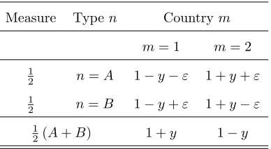
Without loss of generality, suppose country 1 has initial aggregate endowment1 +y. Then, the

endow-ment structure at period 0 can be summarized in Table 1, where superscript m = f1;2g denotes country

endowment structure in either country repeats itself every two periods. Therefore, country 1 is

interna-tionally participation constrained at all even numbered periods 0;2;4; :::;1, even type B with a relatively

lower endowment. At all odd numbered periods 1;3;5; :::;1; country 1 as a borrower is unconstrained in

international …nancial markets.

After the type is known to residents and before the realization of initial aggregate endowment for countries,

a representative resident of any type has expected life time preference

E[u(z)] = 1

2[log(1 +z) + log(1 z)] + 1

2[log(1 z) + log(1 +z)];

wherez represents consumption deviation and denotes discount factor. E[u(z)]is strictly decreasing inz

as depicted in Figure 2. More international risk sharing means higher ex-ante welfare.

4.1

Private Borrowing with Full Commitment Domestically

Because domestic debt contracts are perfectly enforced, di¤erent types in the same country consume the

same amount of goods every period. The consumption pattern in the world is as follow

c1t = 1 +xJ; c1t+1= 1 xJ; for country 1;

c2t = 1 xJ; c2t+1= 1 +xJ; for country 2.

Country 1 is participation constrained in international …nancial market at period0, which implies that the

present value of all future net payments to foreigners when discounted by Arrow-Debreu domestic bond

prices is zero.5

xJ _{y+q y x}J

1 pq = 0: (16)

The price for international bonds today denoted by q is determined by the MRS in countries that are

unconstrained next period. In other words, international bond price can be found in countries whose residents

consume1 +xJ _{today and1 x}J _tomorrow.

q= 1 +x

J

1 xJ: (17)

Andpdenotes the price for domestically traded bonds when the country is participation constrained next

period

p= 1 x

J

1 +xJ:

The price sequences for domestic bonds traded in country 1 and country 2 are

p1 =

8 > <

> :

p; for period0;2;4; :::

q; for period 1;3;5; :::

; (18)

p2 =

8 > <

> :

q; for period 0;2;4; :::

p; for period1;3;5; ::: :

There are two solutions to equation (16). The …rst is autarky, orxJ _{=y; while the second requires q= 1;}

which further impliesxJ ₌1

1+ using equation (17).

4.2

Centralized Borrowing

Consider a world of two centralized economies where government lends and borrows internationally, decides

whether or not to renege on debt owned by the country, and apportions total endowment plus net foreign

capital in‡ow among residents. This government regulation is introduced to help the welfare comparison

between my model and Jeske’s setup. Because of government’s intervention in domestic allocation, one can

aggregate each country into a representative agent with the following consumption pattern

c1_t = 1 +xc; c1_t+1= 1 xc; for country 1;

c2_t = 1 xc; c2_t+1= 1 +xc; for country 2,

wherexc _{is the minimum deviation satisfying country 1’s international participation constraint at timet}

xc= min

z>0fz: log(1 +z) + log(1 z) log(1 +y) + log(1 y)g:

For the problem to be interesting, I am looking for the situation in which some (not full) risk sharing can

be supported across centralized economy. This is only possible given two restrictions on endowment are

satis…ed. The …rst one is

< log(1 +y)

log(1 y); (19)

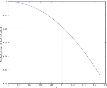
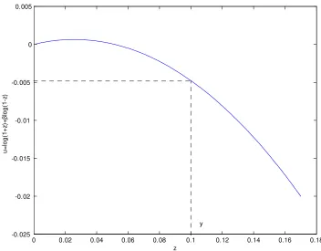
otherwise countries can fully smooth consumption,xc_{= 0 as in Figure 3. The second one is}

> 1 y

1 +y;

or equivalently

y >1

otherwise autarky is the highest utility one can achieve and there is no trade in equilibrium, xc _{=y as in}

Figure 4.

If (19) and (20) are both satis…ed, some international risk sharing can be supported across border. As

can be seen in Figure 5, the risk sharing level in centralized economy turns out to be better than the private

international borrowing with full domestic commitment in section 4.1,

0< xc< 1

1 + < y:

Given thatxJ =1₁₊ ory;I know the following relationship

0< xc< xJ 6y:

4.3

Private Borrowing with Limited Commitment Domestically

Next I remove the assumption of perfect enforcement on domestic debts. Therefore, type A and type B

agents in the same country might have di¤erent consumption allocations. As a result, the allocations in

trade equilibrium alternate not only between di¤erent types within a country but also across countries. By

symmetry, I have

c1A;t = 1 +x+"p; c1A;t+1= 1 x "p; for type A in country 1;

c1B;t = 1 +x "p; cB;t1 +1= 1 x+"p; for type B in country 1;

c2_A;t = 1 x "p_{; c}2

A;t+1= 1 +x+"p; for type A in country 2;

c1_B;t = 1 x+"p_{; c}1

B;t+1= 1 +x "p; for type B in country 2.

The consumption structure implies two possibilities: "p_>0and"p_{= 0:}

"p _{>0means di¤erent types within the same country can not match consumption even though}

interna-tional …nancial markets are accessible, thus Type B agents with a less volatile consumption deviation must

be domestically participation constrained if the country is internationally participation constrained in trade

equilibrium. xand"p _{are jointly determined by three conditions. The …rst two conditions are derived from}

the fact that type A and B in country 1 are internationally participation constrained at the same time. For

discounted by domestic bond prices.

(x+"p) (y+") +q[(y+") (x+"p)]

1 pq = 0for type A; (21)

(x "p_{) (y ") +q[(y ") (x "}p_)]

1 pq = 0for type B.

The third condition says that if type B residents are participation constrained in domestic and international

…nancial markets at the same time, then their continuation values in trade equilibrium and resident’s autarky

must be equalized at some even numbered period.

log(1 +x "p) + log(1 x+"p) = log(1 +y ") + log(1 y+"): (22)

At even numbered period, the international bond priceqequals to the highest MRS across the world,

q= 1 +x+"

p

1 x "p; (23)

the domestic bond price in country 1 is q;6 _{and the domestic bond price in country 2 equals to the lowest}

MRS within 2,

p= 1 x "

p

1 +x+"p:

As a result, the price sequences for domestically traded bonds are the same as (18) in section 4.1. There is

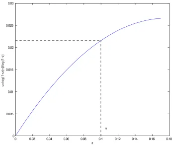
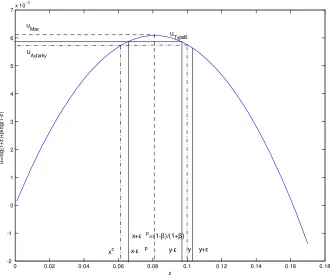
a unique solution to (21) and (22). The optimal solution requiresq= 1;which further impliesx+"p= 1₁₊

using (23) and "p _{is determined implicitly by equation (22). Given that y is large relative to ", as well as}

"p>0;I know xc < x "p< 1₁₊ from Figure 6.

On the other hand"p _{= 0indicates international …nancial markets help di¤erent types within the same}

country to match consumption every period. Therefore, no one is constrained domestically and the MRS

is equalized in that country. x is then determined by (21). Use (23) again and get the optimal solution

x=1₁₊ ; "p= 0:

4.4

A Comparison of Risk Sharing

Now I can compare the extent of self-enforcing deviation from consumption smoothing in the above three

scenarios. In section 4.1 (scenario 1), both types have the same deviation xJ ₌ 1

1+ or y. In section 4.2

6_{In contrast to the formal model, the MRS is not equalized within country 1 at period0in this simple example.}

q= 1 +x+"

p

1 x "p >

1 +x "p

1 x+"p; if" p_>0:

(scenario 2), both types have the same deviationxc_{. In section 4.3 (scenario 3), either both types have the}

same deviationx=1₁₊ or type A has deviationx+"p₌ 1

1+ while type B has deviationx "p< 1 1+ . To

summarize,

0 < xc < x+"p6xJ6y; for type A;

0 < xc < x "p6xJ6y; for type B.

Adding domestic enforcement problem rules out the autarky solution, xJ _{= y; in scenario 1. For both}

types, risk sharing levels are weakly improved. If type A and B cannot match consumption, then B’s

international risk sharing level is strictly improves by scenario 3, though the increment is smaller than the

one by centralization in scenario 2.

In conclusion, given the endowment structure withyrelatively larger than", I …nd the domain 1₁₊y_y; log(1+_log(1 y_y)₎

for discount factor where scenario 2 is always welfare superior than 1 or 3 and 3 is strictly better than 1.

This is the case I studied in section 3. What happens if the discount factor is high enough, 2h log(1+_log(1 y_y)₎;1i;

then one will observe complete international risk sharing in scenario 2 which can never be an equilibrium

allocation in scenario 1 and 3. If agents are extremely impatient, 2h0;1₁₊y_yi;then both scenario 1 and 2

lead to the same equilibrium of autarky with complete domestic risk sharingxc _=xJ_{=y. Scenario 3 would}

result in autarky with no domestic risk sharing,x=yand "p _{=";which is worse than scenario 1 and 2.}

5

Conclusion

I have developed an open economy model with heterogeneous residents in each country sharing risk across

and within border. Risk of repudiation is pervasive in all debt contracts including both international and

domestic ones. The model and analysis is built on Jeske’s private international borrowing model except

relaxing his assumption that domestic debt contracts are perfectly enforceable. In this paper, besides the

di¤erence in price, international debt contracts also di¤er from domestic ones in punishing strategy defaulters.

International debt defaulters are excluded only from international …nancial markets while domestic debt

defaulters are denied from all …nancial markets.

The main contribution of this paper is to show that an economy with pervasive enforcement problem does

better in international capital markets than an economy with enforcement problem on foreign debts alone.

model and strictly harsher for some types with smoother endowment overtime. Thus, more international

borrowing and higher welfare can be supported for those lucky types of residents. Intuitively, capital control

internalizes the externality of individual’s default decisions while pervasive commitment problem mitigates

the negative externality. The domestic bond pricing rules change in respond to the domestic credit crisis. In

my setup, domestic interest rate equals to the reciprocal of the lowest MRS in countries that are participation

constrained internationally. This overthrows the well established argument that interest rate should be the

lowest to induce repayment in an environment without legal enforcement on …nancial contracts. This result

is due to the crucial ingredient of my model: in equilibrium domestic debt default can never happen without

international debt default. Although there is commitment problem within border, domestic debt repayment is

secured by preventing international debt default. For countries whose international participation constraint

is super‡uous, their domestic interest rate equals to prevailing international interest rate as in previous

References

[1] Alvarez, Fernando, and Urban J. Jermann. 2000. “E¢ciency, Equilibrium, and Asset Pricing with Risk

of Default.”Econometrica68 (4): 775-798.

[2] Alvarez, Fernando, and Urban J. Jermann. 2001. “Quantitative Asset Pricing Implications of

Endoge-nous Solvency Constraints.”The Review of Financial Studies 14 (4): 1117-1151.

[3] Azariadis, Costas, and Luisa Lambertini. 2002. “Excess Asset Returns with Limited Enforcement.”The

American Economic Review 92 (2): 135-140.

[4] Broner, Fernando, and Jaume Ventura. 2009. “Globalization and Risk Sharing.”NBER Working Papers

12482, National Bureau of Economic Research.

[5] Bulow, Jeremy, and Kenneth Rogo¤. 1989. “Sovereign Debt: Is to Forgive or Forget?” American

Eco-nomic Review 79 (1): 43-50.

[6] Hellwig, Christian, and Guido Lorenzoni. 2007. “Bubbles and Self-Enforcing Debt.” Econometrica 77

(4):1137-1164.

[7] Jeske, Karsten. 2006. “Private International Debt with Risk of Repudiation.”Journal of Political

Econ-omy 114 (3): 576-593.

[8] Jeske, Karsten. 2001. “Private International Debt with Risk of Repudiation.”Working Papers 2001-16,

Federal Reserve Bank of Atlanta.

[9] Kehoe, Timothy, and David Levine. 1993. “Debt-Constrained Asset Markets.” Review of Economic

Studies60 (4): 865–888.

[10] Kehoe, Patrick J., and Fabrizio Perri. 2004. “Competitive Equilibria with Limited Enforcement.”

Jour-nal of Economic Theory 119 (1): 184-206.

[11] Kehoe, Patrick, and Fabrizio Perri. 2002. “International Business Cycles with Endogenous Incomplete

Markets.”Econometrica 70 (3): 907-928.

[12] Kocherlakota, Narayana. 1996. “Implications of E¢cient Risk Sharing without Commitment.” Review

[13] Uribe, Martin. 2006. “On Overborrowing.”American Economic Review 96 (2): 417-421.

[14] Wright, Mark. 2006. “Private Capital Flows, Capital Controls, and Default Risk.”Journal of

A

Appendix

A.1

Proof of Proposition 1

Imagine an Arrow-Debreu setup in which there exists a domestic …nancial market at period0for all kinds of

bonds that mature at any future period. DenotePm₍ r_{) =P}m₍ r 1

)pm₍ r 1

; r) = r Y

s=0

pm₍ s_{)the forward}

price for ar-period matured domestic contingent bond at period0;wherer2(0;1)andPm₍ 0

) =pm₍ 0 ) =

1: The proof proceeds in three steps:

Step 1: _{Rede…ne the resident’s international autarky problem (RIA) started at} t_{as follow}

Vm

n ( t; bmn( t)) max

fcm

n( r)gr2[t;1)

1

X

r=t

r t X

r_j t

( rj t)U(cm

n( r)); (RIAF)

subject to the summation of all future budget constraints after history t discounted to period0

1

X

r=t

X

r_jt

Pm₍ r_)cm

n( r) =

1

X

r=t

X

r_jt

Pm₍ r_)em

n( r) +Pm( t)bmn( t);

and the participation constraint in domestic …nancial markets

1

X

s=r

s r X

s_jr

( sj r)U(cm_n( r))>Am_n( r);

with

bm_n( t)andPm( r)given,

for all histories twithr2[t;1):

Lemma 1 The rede…ned resident’s international autarky problem (RIAF_{) has a unique maximum solution.}

Proof. Prove by contradiction. Suppose there are two di¤erent optimal solutions to problem (RIAF):

n

cm;D_n;1 ( r)

o

r2[t;1) and

n

cm;D_n;2 ( r)

o

s2[t;1): Create another consumption allocation

n

cm;D_n;3 ( r)

o

r2[r;1) as a

linear combination of the above two, i.e.,

cm;D_n;3 ( r) = cm;D_n;1 ( r) + (1 )cm;D_n;2 ( r)

for any 2(0;1) and history r withr2[t;1): Thus, ncm;D_n;3 ( r)o

r2[t;1) is both a¤ordable and individual

rational since strictly concave utility function implies

1

X

s=r

s r X

s_jr

( sj r)U(cm;D_n;3 ( s))>

1

X

s=r

s r X

s_j r

for all histories r withr2[t;1): But ncm;D_n;3 ( r)o

r2[t;1) makes one strictly better o¤ at the …rst place if

one setsr=t, which contradicts with the assumption thatncm;D_n;1 ( r₎o

r2[t;1) and

n

cm;D_n;2 ( r₎o

t2[t;1) are the

optimal solutions.

Step 2: _ForFm

n (

t₎₂

R;de…ne another optimization problem (RPF_{) as an augmented version of (RIA}F₎

W_nm;F( t; bm_n( t); F( t)) max

fcm

n(r)gr2[t;1)

1

X

r=t

r tX

r_jt

( rj t)U(cm_n( r)); (RPF₎

subject to the summation of all future budget constraints after history t discounted to period0

1

X

r=t

X

r_jt

Pm( r)cm_n( r) =

1

X

r=t

X

r_j t

Pm( r)em_n( r) +Pm( t)bm_n( t) +F_nm( t);

and the participation constraint in domestic …nancial markets

1

X

s=r

s r X

s_jr

( sj r)U(cm_n( s))>Am_n( r);

with

bmn( t); Fnm( t)andPm( r)given,

for all histories r _withr2[t;1):

Consider all histories tand initial bond holdingsbm

n( t)witht2[0;1):By de…nition, the value function of problem (RIAF_{) equals to the value function of problem (RP}F_{) givenF}m

n ( t) = 0:

V_nm( t; bm_n( t)) =W_nm;F( t; bm_n( t);0);

If one de…nes

F_nm( t_{) =}

1

X

r=t

X

r_j t

Pm( r₎ 2

4f_nm( r₎ X

r+1

q( r_;

r+1)fnm( r; r+1)

3

5;

then the continuation value of the original resident’s problem (RP) at tequals to the value function of the

newly de…ned problem (RPF_).

1

X

r=t

r tX

r_jt

( rj t)U(cm_n( r)) =W_nm;F( t; bm_n( t); F_nm( t)):

But this equality is true only if the international participation constraints (4) in (RP) are also satis…ed in

(RPF_).

1

X

r=t

r t X

r_j t

Substitute both sides of the constraints for value functions in (RPF_{) to get}

W_nm;F( t; bm_n( t); F_nm( t))>W_nm;F( t; bm_n( t);0):

SinceWm;F

n ( t; bmn( t); )is strictly increasing in Fnm( t);the above inequality further implies

Fnm( t)>0:

What is more, if (4) holds with equality, then Fm

n ( r) = 0. By now, the reasoning su¢ces to prove the following lemma 2

Lemma 2 For allm; nand twith t2[0;1); the international participation constraint (4) at t implies

1

X

r=t

X

r_j t

Pm( r)

2

4f_nm( r) X

r+1

q( r; r+1)fnm( r

; r+1) 3

5>0:

Moreover, if (4) holds with equality at t, then

1

X

r=t

X

r_j t

Pm( r)

2

4f_nm( r) X

r+1

q( r; r+1)fnm( r; r+1) 3

5= 0:

Step 3: _{Now I am ready to prove proposition 1. For some n; m and} t _{with t 2 [0;1);} m

n( t) > 0

implies that the international participation constraint of type n residents in country m holds with

equal-ity at t_{: Lemma 2 concludes F}m

n ( t) = 0: By de…nition, the consumption allocation cm;Dn ( r) r2[t;1)

solves problem (RIA) started at t and the other one fcm

n( r)gr2[0;1) solves problem (RP) at period 0.

That is to say, cm;D

n (

r₎

r2[t;1) solvesW

m;F

n (

t

; bm

n(

t₎

;0) and fcm

n(

r_)g

r2[t;1) fcmn(

r_)g

r2[0;1) solves

Wm;F

n ( t; bmn( t); Fnm( t)): SinceFnm( t) = 0;these two optimal allocations both solveWnm;F( t; bmn( t);0), i.e., they both solve the resident’s international autarky problem (RIA) and its rede…ned problem (RIAF₎

with value functionVm

n ( t; bmn( t)):Finally, by Lemma 1, the optimization problem (RIAF) having unique solution proves thatcm;D

n (

r_)and

cm

n(

r_{)are identical at all histories} r _with

r2[t;1):

A.2

Proof of Proposition 2

In equilibrium, bond prices are determined by (13) and (14) for all histories( t; t+1)witht2[0;1). 8

> <

> :

p( t; t+1) = U

0₍

c( t

;t+1))

U0_(c(t₎₎ ( t+1j t)

1+A2 (1+ ( t;t+1))A1 1+A3 ;

q( t; t+1) = U

0_(c( t_; t+1))

where

A1 = ( t; t+1) t 1

U0(cD( t; t+1))

U0_(c( t_;

t+1))

1 ( t; t+1)

;

A2 =

t+1

X

s=0

X

t_; t+1js

( s) s (

t

; t+1j s) ( t; t+1)

;

A3 =

t X

s=0

X

t_js

( s) s (

t_j s₎

( t₎ :

The proof shows in three steps how the interaction between international and domestic bond prices makes

di¤erent types reach their upper limits of international borrowing at the same time.

Step 1: _{Consider the international bond pricing rule (14), the Lagrange multipliers imposed on the}

international participation constraints must be non-negative.

( t; t+1)>0)

A2=A3+ ( t; t+1) t 1

1 ( t; t+1)

>A3;

and

A2=A3 if ( t; t+1) = 0:

Therefore, the international bond price represents the highest MRS among all types in all countries.

q( t; t+1)>

U0_(c( t_;

t+1))

U0_(c( t₎₎ ( t+1j t); with equality iif mn( t; t+1) = 0: (A.1)

Step 2: _{Consider the domestic bond pricing rule (13) in any country. Substitute all theA’s and rearrange}

p( t; t+1) =

U0_(c( t_;

t+1))

U0_(c( t₎₎ ( t+1j t)

8 > > > < > > > :

1 + (1

U0(cD( t

;t+1))

U0_(c( t_;

t+1)) )

( t

;t+1) t 1

(t_; t+1)

U0(cD(t

; t+1))

U0_(c( t_;

t+1))

( t

;t+1) ( t;t+1) t 1

(( t_; t+1))

1 +Xt

s=0

X

t_js

( s) s (₍tjt₎s)

9 > > > = > > > ; :

For some typeninm;if one observes m

n(

t

; t+1) = 0;then the domestic bond price inmis determined by

n’s MRS.

pm( t; t+1) =

U0(cm

n(

t

; t+1))

U0_(cm

n( t))

If one observes m

n( t; t+1)>0 instead, thencm;Dn ( t; t+1) =cmn( t; t+1)by proposition 1. The relation-ship between domestic bond price inm andn’s MRS is

pm( t; t+1) =

U0_(cm

n( t; t+1))

U0_(cm

n(

t₎₎ ( t+1j t)

2 6 6 6 41 m

n( t;t+1) mn( t;t+1) t 1

(( t_; t+1))

1 +Xt

s=0

X

t_j s

m

n( s) s

( t_js₎

(t₎

3

7 7 7

5: (A.2)

The Lagrange multipliers imposed on domestic participation constraints in problem (RIA) must be

non-negative.

v_nm( t; t+1)>0)

pm₍ t_;

t+1)6

U0_(cm

n( t; t+1))

U0_(cm

n(

t₎₎ ( t+1j t); with equality ifvmn( t; t+1) = 0: (A.3)

Step 3: _If m

n(

t

; t+1)>0for some typenresidents in countrym;then (A.1) and (A.3) together ensure

that the international bond price is strictly greater than the domestic one inm:

q( t_;

t+1)>

U0(cm

n(

t

; t+1))

U0_(cm

n( t))

>pm( t_;

t+1))

q( t; t+1)> pm( t; t+1):

This strict inequality, the other way around, implies that multipliers m

n( t; t+1)are positive for all types inm as well.

q( t; t+1)> pm( t; t+1))

U0_(cm

n( t; t+1))

U0_(cm

n(

t₎₎ ( t+1j t)

1 +Am

n;2

1 +Am

n;3

> U

0_(cm

n( t; t+1))

U0_(cm

n(

t₎₎ ( t+1j t)

1 +Am

n;2 1 + mn(

t

; t+1) Amn;1 1 +Am

n;3

)

1 + m

n(

t

; t+1) mn( t

; t+1) r 1

1 ( t; t+1j t)

>0)

1 + mn( t; t+1) nm( t; t+1)>0:

Since m

n(

t

; t+1)>0 for allnin m;I have

m

n( t; t+1)>0; for alln; m:

A.3

Proof of Proposition 3

Given m

n(

t₎

>0for somen; mat twitht2[0;1);the international participation constraint in resident’s

problem is binding at t.

1

X

r=t

r t X

r_j t

where cm

n( r) and bmn( t) are the optimal consumption at r and the optimal domestic bond holdings at t _{in problem (RP). The value function}

Vm

n (

t

; bm

n(

t_{))of problem (RIA) started at} t_{a¤ects the optimal}

consumption allocation after tin problem (RP) through this binding constraint. In addition, m

n( r)>0

for the same n and m above with r 2 [t;1) implies the domestic participation constraint in resident’s

international autarky problem is bind at r:

1

X

s=r

s r X

s_jr

( sj r)U(cm;D_n ( s; t; bm_n( t))) =Am_n( r);

wherecm;D

n (

s

; t; bm

n(

t_{))denotes the optimal consumption at} s_{in problem (RIA) started at} t_{with initial}

domestic bond holdingsbm

n( t). This equation implicitly de…nesbmn( t) =B m

n( t):

A.4

Proof of Proposition 4

By lemma 2 and proposition 3, the international participation constraint (4) at t with t2 [0;1)implies

the following set of inequality and equality constraints

8 > > > > > > < > > > > > > : X1

r=t

X

r_j t

Pm₍ r₎ 2

4fm

n ( r)

X

r+1

q( r; r+1)fnm( r; r+1) 3

5>0;

bm

n(

t

; t+1) =B m

n(

t

; t+1)if mn( t

; t+1)>0 and

m

n( r; r+1)>0for some r withr2[t;1):

(A.4)

The proof proceeds in the following three steps: de…ne, solve and compare.

Step 1: _{For all histories} t_{witht2[0;1);replacing (4) in problem (RP) with weaker constraints (A.4)}

creates an alternative (convex) resident’s problem (RPa_).

max

fcm

n( t);bmn( t;t+1);fnm( t;t+1)gt2[0;1)

1

X

t=0

tX

t

( t)U(cm_n( t)); (RPa₎

subject to the budget constraint

em_n( t) +bm_n( t) +f_nm( t)

> cm_n( t) +X

t+1

pm( t; t+1)bmn( t; t+1) + X

t+1

q( t; t+1)fnm( t; t+1); (A.5)

the weaker version of participation constraint in international …nancial market

1

X

r=t

X

r_j t

Pm( r)

2

4f_nm( r) X

r+1

q( r; r+1)fnm( r; r+1) 3