Towards Analysis of Vertical Structure of Industries: a method and its application to U S industries

Munich Personal RePEc Archive

Towards Analysis of Vertical Structure of

Industries: a method and its application

to U.S. industries

Sadao, Nishimura

15 December 2010

Online at

https://mpra.ub.uni-muenchen.de/27464/

Towards Analysis of Vertical Structure of Industries:

a method and its application to U.S. industries

Sadao Nishimura

Abstract

In this paper we present a method to analyse vertical structure of industries. A product of an industry has a

hi-erarchical value structure with layers, each of which consists of value added injected by various production stages

(current and previous) of various industries. This vertical structure makes it possible to measure value added (VA)

levels (vertical positions) of VA receivers (stages of use industries), while products of supply industries and their

value added flow into these stages of industries which have respective VA levels. These flows are value added

contributions by supply industries. By calculating each industry’s VA contributions and corresponding target VA

levels, it is possible to evaluate vertical structure of industries in the whole economy. We applied this method to

1998–2008 U.S. Input-Output Tables. Resulting average VA contribution levels and graphs of VA contributions

are displayed.

Keywords: vertical structure, value added, supply, use.

JEL Classification Codes: C61, D57

1

Introduction

A phenomenon called vertical specialization has attracted a great deal of attentions for recent decades. This

phenomenon is referred to as several different names such as fragmentation, disintegration of production,

multi-stage production, intra-product specialization, and so on1_.

Probably one of the reasons of many arguments raised on this problem is the controversy in the United States

over “offshoriong.” That is, on the one hand there are many who insist the offshoring is prone to exporting many

domestic jobs abroad to other (more often than not, emerging or developing) countries, and have domestic workers

lose their opportuinities to work. On the other hand, many economists defend the offshoring as a variant of

international trade, and therefore it is beneficial for both countries of job offers and receivers.

Obviously, among the factors which brought about offshoring is siginificant progress in information and

com-munication technologies (ICT) in recent years. Typical services had been difficult to be traded between distant

places as they needed to be produced just when and where they were consumed. However, recent conspicuous

technological progress particularly in digitaization of information made it possible to exchange services between

distantly separated firms and individuals. The UNCTAD, for example, prepared a chapter in its World Investment

Report 2004 ([6]) to analyse this problem from various points of view using vast range of facts and data.

Arguments in the literature, however, do not seem to have converged into standard models or theories. One of

the reasons for this situation is, according to my view, the lack of systematic methods in dealilng with data. Data

and documents are not in short supply. On the contrary, many researchers refer and cite a great deal of data, facts,

and anecdotes in their studies.

One of the key to study offshoring is how to analyse the structure of industries. If we can show empirically the

effects of offshoring on the industrial structure of an economy (e.g. American economy), theoretical discussion

will probably become integrated into some consistent models based on actual data, and by this reason, empirical

studies will also develop further.

The problem is not easy, however. It seems that offshoring phenomenon is, for the industries in question,

essentially a microeconomic problem. Therefore, data related to offshoring may be also microscopic, which are

essentially connected to individual firms engaging in offshoring. On the other hand, however, if offshoring has

some effects on the industries’ structure at all, it will probably have to be clarified by examining the position of the

industry in the whole economy, particularly by examining changes in their position in the vertical structure of total

industry.

This paper is an attempt towards this research direction. We use the Input-Output data and analysis in order to

investigate the vertical structure of an economy’s industries. By making out the concept of ‘vertical structure’ of

industries, we will become able to apply this concept in examining the effects of offshoring (or other phenomena)

on the structure of industries.

The basic idea of this paper is as follows. The fundamental equation in input-output alaysis is:

X=AX+Y,

whereXis a vector of total production,Y of final demand, andAis a direct input requirement coefficient matrix.

By solving this equation forX, we have

X=LY=(I+A+A2+. . .)Y. (1)

Lis the well-known Leontief inverse matrix, and (I+A+A2_{+. . .) is an expression in its expanded form. This}

expansion form is the starting point of our discussion.

The first term of the right-hand part of the equation (IY = Y) indicates the products of the final production

stage (stage-0) of the economy. To produce stage-0 products, the economy has to produce inputs which correspond

to the second term (AY), the products of stage-1. This process traces back to infinite stage numbers2.

The stage numberλofAλY indicates how ‘old’ its production process is and how long ago the corresponding

value added are embedded in these inputs. In other words, the various stages’ value added are piled up to form

the total value of final productsY. This forms a hierarchy structure, which somewhat resembles growth rings of

trees. If we can analyse changes in this growth ring structure raised by some impacts, we can find the effects of the

impacts on the structure of industries in question.

2_{In order to avoid confusions, we use the following terminology. All production stages are assigned a non-negative integer starting from 0.}

The last stage, which is not acutually a production process, is absorption by final demand and assigned 0. One stage before stage-0 is stage-1,

which produces stage-0 products that are absorbed by stage-0 activity (final demand), and uses stage-1 products as inputs, which are products

The value added hierarchy structure of industries or products can also be utilized in somewhat different

per-spective. (1) shows production ofX, which is larger than final demandY, needs to be produced to fullfil the final

demand. Then, total amount of each product is distributed to various stages (from stage-0 to stage-∞) of vari-ous industries (products) in order to support production of varivari-ous products. If an industry’s product is mainly

distributed into rather lower-numbered stages of production, we presume the industry is contributing in near final

demand stages. That industry can be called a (relatively) downstream industry. If the other is the case, it can be

called an upstream one.

A product of any industry is a heap of value added injected in various production stages of (use) industries. If

we can evaluate the height of the value added whithin the total value added stratum of the product, then we can also

evaluate the height of the contribution performed by (supply) industries sending their value added to destinations.

Accordingly, it will become able to calculate the vertical position of each industry within the economy-wide

structure of industries. This method presumes the stage-0 (producing final goods to final demand) is at the highest

position in the vertical hierarchy, and the earliest stage-∞is at the lowest (ground)3_.

In the next section, the formal model of vertical structural analysis is presented. It is applied to some industries

of the United States, particularly those closely related to ‘offshoring’.

2

A Method to Analyse Vertical Structure of Industries

2.1

Value Added Hierarchy of Products of Use Industries

Each industry produces its peculiar product and supplies it to many other industries and final demand. When our

attention is centered on this aspect of an industry, we call it a supply industry. At the same time, each industry

uses various intermediates supplied by other industries which are necessary for its production processes. When we

pick up this aspect of an industry, we call it a use industry. That is, industries have two different relationships with

3_{Here is some obvious problem. For example, we include both consumption goods and investment goods in final goods by statistical}

convention. But investment goods (capital goods) can be considered as intermediate goods in a long roundabout production process. For now

others. In this section we will discuss the aspect of use industry4_.

The total value of product of a use industry constitutes piled layers of the value added created in a myriad

of production process chains which are in the end connected to the product of this use industry. Intermediates

produced in preceding production processes are absorbed into some production stages, which, in turn, send their

products as intermediates to later stages. Such production process chains intersect, get intermingled, and after a

long travel reach their last stage. This is the final products abrosbed by final demand.

Let us consider the composition of value added which a use industry’s product fills with.

First, we assume there is no need to distinguish between a use industry and its product5_{. Each product is}

produced by only one use industry, and each industry produces only one product. Then, assumePis a column

vector of product prices, andV is a column vector of direct value added of use industries. About product value

construction we have the price model expression of input-output relations.

P′=P′A+V′.

The right-hand side of this equation is the cost of inputs per unit of output including value added. If we take the

unit of each product equal to the amount the monetary unit can purchase, andvbe the rate of value added in the

product value, we have

u′=u′A+v′. (2)

whereuis a column vector of 1’s (u=(1,1, . . . ,1)′). Using the expansion form of Leontief inverse matrix, we get

the following expression.

u′=v′(I+A+A2+· · ·). (3) The first term in the right-hand side parenthesesI(=A0_{) indicates that unit amount of each product is used by}

stage-0. The power 0 ofAmeans the stage number of the process, which actually is not a production process but

the activity of abrosption (purchase) by final demand. The second termArepresents intermediate inputs required

by the production stage-1 which is to produce unit amount of each product to deliver to the final demand (stage-0).

In generalAλ_{is intermediate inputs required by the production stage-λwhose products are delivered to the next}

4_{Usage of these terms might be somewhat confusing, but these some commonality with the words “supply” and “use” used in the}

commodity-by-industry approach in input-output analysis.

production stage-(λ−1) as intermediate inputs. As the right-hand side of (3) is the sum of total amount of products premultiplied byv′, the equation means the sum of all value added poured into the unit of final product equals 1

for each product.

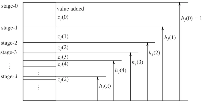
Let us take the product j, and examine the hierarchical structure of its value added. The value added in a unit

amount of (final) product jinjected by inputiat production stage-λis shown by (i,j) element ofv′Aλ, orvia

(λ)

i j

6_.

Total value added injected by all inputs at the production stageλiszj(λ)= ivia

(λ)

i j . Then,

1=zj(0)+zj(1)+· · ·+zj(λ)+· · ·.

The larger the stage numberλis, the earlier is the production stage. That means, the largerλis, the smaller is the

value added accumulated in product jthrough successive stages up to stage-λ.

zj(0)

zj(2)

zj(3)

zj(4) ..

.

zj(λ) ..

.

hj(0)=1

zj(1) hj(1)

hj(2)

hj(3)

hj(4)

hj(λ) stage-0

stage-1

stage-2

stage-3

.. .

stage-λ

value added

Figure 1: Vertical Value Added Structure of product j

Figure 1 shows this hierarchical value added structure for product j. On the top of the layers lies the value

added to the product jabsorbed in the last stage of production. The second layer is the value added absorbed in the

second last stage, and so on. In general, inputs to production stage-λhave value equal to the sum of value added

layerzj(λ) and below (zj(λ)+zj(λ+1)+· · ·), and the immediate upper layerzj(λ−1) is the value added newly created at the production stage-λ.

We now define thevalue added level(or simplyVA level) of a production stage. This is a concept of height

of the value added layer corresponding to the stage in question. For example, the VA level of stage-λ,hj(λ), is

6_a(λ)

expressed as

hj(λ)=zj(λ)+zj(λ+1)+zj(λ+2)· · ·, wherehj(λ)≥hj(λ+1), hj(0)=1 andhj(∞)=0.

Leth(λ)=(h1(λ), . . . ,hj(λ), . . . ,hn(λ))′, wherenis the number of products or industries. Then we have

h′(λ)=v′(Aλ+A(λ+1)+A(λ+2)+. . .)

=v′(I+A+A2+. . .)Aλ

=u′Aλ. (4)

That is, the VA level of stage-λof productj,hj(λ), is the column sum ofj-th column of matrixAλ_{. If jis different,}

hj(λ) is not generally the same. It is evident thath′(λ+1)=h′(λ)A.

Then let our dicussion concentrate on individual product or industry. Take a product (or industry) j. The VA

level of the stage-λof product jis the j-th element of the row vectorh′

(λ) = u′_Aλ_{, or} ia

(λ)

i j . In this stage-λ,

an individual producti contributes in value added formation by the amount ofvia

(λ)

i j . Let a hat over a vector ˆx

denote a diagonal matrix with elements ofxalong the main diagonal. Then j-th column vector of ˆvAλ_represents

contributions ofn(different) products in product j’s stage-λ.

Usinga(_{i j}λ)’s (i=1, . . . ,nandλ=0, . . . ,∞), we construct the following matrix with infinite rows. This matrix is related to use industry j, and we can constructnkinds of similar matrices for different use industries.

A(j)=

⎛ ⎜ ⎜ ⎜ ⎜ ⎜ ⎜ ⎜ ⎜ ⎜ ⎜ ⎜ ⎜ ⎜ ⎜ ⎜ ⎜ ⎜ ⎜ ⎜ ⎜ ⎜ ⎜ ⎜ ⎜ ⎜ ⎜ ⎜ ⎜ ⎜ ⎜ ⎜ ⎜ ⎜ ⎜ ⎜ ⎜ ⎜ ⎜ ⎜ ⎜ ⎜ ⎜ ⎜ ⎜ ⎝

0 0 . . . 1 . . . 0

a1j a2j . . . aj j . . . an j ..

. ... ... ... ... ...

a(₁λ_j) a(₂λ_j) . . . a(_{j j}λ) . . . a(_{n j}λ)

..

. ... ... ... ... ... ⎞ ⎟ ⎟ ⎟ ⎟ ⎟ ⎟ ⎟ ⎟ ⎟ ⎟ ⎟ ⎟ ⎟ ⎟ ⎟ ⎟ ⎟ ⎟ ⎟ ⎟ ⎟ ⎟ ⎟ ⎟ ⎟ ⎟ ⎟ ⎟ ⎟ ⎟ ⎟ ⎟ ⎟ ⎟ ⎟ ⎟ ⎟ ⎟ ⎟ ⎟ ⎟ ⎟ ⎟ ⎟ ⎠

(5)

The first row ofA₍j) is the transpose of j-th column of identity matrix orA0, the second is j-th column ofA, the third is j-th column ofA2, and so on. In general theλ-th row is the transpose of the j-th column ofAλ. Elements

ofA(j), thus, exhaust direct and indirect inputs to use industry jto produce product j. Each element ofA(j)’s

i-th column shows the amount of product supplied by industryito various stages of industryj. Finally, the sum of

A(j)’s (λ+1)-th row elements is VA levelhj(λ) of the stage-λ hj(λ)= ia

(λ)

i j

Next, we postmultiplyA(j) by ˆvto get:

V(j)=

⎛ ⎜ ⎜ ⎜ ⎜ ⎜ ⎜ ⎜ ⎜ ⎜ ⎜ ⎜ ⎜ ⎜ ⎜ ⎜ ⎜ ⎜ ⎜ ⎜ ⎜ ⎜ ⎜ ⎜ ⎜ ⎜ ⎜ ⎜ ⎜ ⎜ ⎜ ⎜ ⎜ ⎜ ⎜ ⎜ ⎜ ⎜ ⎜ ⎜ ⎜ ⎜ ⎜ ⎜ ⎜ ⎝

0 0 . . . vj . . . 0

a1jv1 a2jv2 . . . aj jvj . . . an jvn ..

. ... ... ... ... ...

a(₁λ_j)v1 a(₂λ_j)v2 . . . a(_{j j}λ)vj . . . a(_{n j}λ)vn ..

. ... ... ... ... ...

⎞ ⎟ ⎟ ⎟ ⎟ ⎟ ⎟ ⎟ ⎟ ⎟ ⎟ ⎟ ⎟ ⎟ ⎟ ⎟ ⎟ ⎟ ⎟ ⎟ ⎟ ⎟ ⎟ ⎟ ⎟ ⎟ ⎟ ⎟ ⎟ ⎟ ⎟ ⎟ ⎟ ⎟ ⎟ ⎟ ⎟ ⎟ ⎟ ⎟ ⎟ ⎟ ⎟ ⎟ ⎟ ⎠

(6)

Elements of V(j) represent amounts of value added allocated to various stages of use industry jfrom various supply industries. For example,a(_{i j}λ)vi, (λ+1,i)-element ofV(j), is the amount of value added conveyed from supply industryito use industry j’s stage-λ.

V(j) shows the most detailed vertical structure of value added embedded in use industry j’s product.

2.2

Value Added Contributions by Supply Industries

Next, we deal with the other aspect of inter-industry relationship: supply of value added by supply industries.

Every use industry produces its particular product by directly and indirectly absorbing value added created in

various supply industries. Then it sells a part of its output to final demand and the rest to various use industries as

their intermidiate inputs. This is the role of supply industry each industry performs in the economy’s input-output

network.

LetXi(i=1, . . . ,n) be the total amount of production in (supply) industryi, or producti, andXbe the column

vector of those outputs (X=(X1, . . . ,Xi, . . . .Xn)′). Similarly, final demand vector is denoted byY =(Y1, . . . ,Yn)′.

Then we have the following basic equation of input-output analysis:

X=AX+Y,

whereAis the direct requirement coefficient matrix as before. This equation can be expressed as ˆXu=AXuˆ +Xˆy,

wherey=Xˆ−1_{Y. Then substitutingB=Xˆ}−1_{AXˆforA. we obtain:}

u=Bu+y. (7)

(i,j) element ofB,bi j= 1

Xi

ai jXj, represents the fraction of productiallocated to use industry jin the total output

direct allocation matrix7_{. Note thatB}λ_=Xˆ−1_Aλ_Xˆ.

We obtain the following from (7):

u=(I−B)−1y=(I+B+B2+. . .)y. (8)

urepresents total outputs of industries normalized to 1’s. The first term of the right-hand sideIy(=y) is the part of

the total output allocated to final demand. The second termByis the part of the output allocated to the stage-1 of

use industries. In general, the (λ+1)-th termBλ_{yis the part of the output allocated to the stage-λof use industries.}

(8) shows the allocation of total output of supply industries among the different stages of different use industries.

Pay attention to the difference between (3) and (8). (3) shows the value added hierarchical structure of use

industries, so focus is on use industries. (8) shows the allocation of supply industries’ products, here focus is on

supply industries.

All elements of the right-hand side ofi-th row of (8) is allocations of the same producti. But, the rate of (direct)

value added is the same for all outputs produced in industryi, the allocating fractions of value added is the same as

those of quantity of producti. Thus the allocation matrixBof outputs is also an allocation matrix of value added.

One point needs to be discussed. Usually direct requirement coefficientsai j’s are considered technologically

constant. Then Leontief inverse matrix (I−A)−1 _=(I+A+A2_{+. . .) is also a constant matrix. However, since}

X=(I+A+A2_{+. . .)Yand final demandYmust be considered a variable,Xcannot be considered constant. That,}

in turn, means thatB =Xˆ−1AXˆ cannot be considered a constant matrix, either. This issue is known as the “joint

stability” problem. IfAis constant,Bin general cannot remain constant. But this issue will not exert damaging

effect on our analysis. A purpose of our analysis is to clarify the existing vertical structure of industries, not to

seek structural characteristics invariant over time. We are more interested in changes in coefficientsbi jofBthan

in their constancy.

As in the previous section, we decompose the expression (8) to make another form of matrix like (5). Consider

the right-hand side of (8). Decompose (λ+1)-th vector,Bλ_{y, by substituting ˆyforyto build a matrixB}λ_{yˆ. Then}

extract itsi-th row. Denote this row vector byc(_iλ)(=(b_i(₁λ)y1,b_i(λ₂)y2, . . . ,b_in(λ)yn) ). Corresponding toλ=0,1, . . . ,∞

we have infinite such row vectors. By arranging these row vectors we construct the following matrixC(i).

C(i)=

⎛ ⎜ ⎜ ⎜ ⎜ ⎜ ⎜ ⎜ ⎜ ⎜ ⎜ ⎜ ⎜ ⎜ ⎜ ⎜ ⎜ ⎜ ⎜ ⎜ ⎜ ⎜ ⎜ ⎜ ⎜ ⎜ ⎜ ⎜ ⎜ ⎜ ⎜ ⎜ ⎜ ⎜ ⎜ ⎜ ⎜ ⎜ ⎜ ⎜ ⎜ ⎜ ⎜ ⎜ ⎜ ⎝

c(0)_i

ci .. .

c(_iλ)

.. . ⎞ ⎟ ⎟ ⎟ ⎟ ⎟ ⎟ ⎟ ⎟ ⎟ ⎟ ⎟ ⎟ ⎟ ⎟ ⎟ ⎟ ⎟ ⎟ ⎟ ⎟ ⎟ ⎟ ⎟ ⎟ ⎟ ⎟ ⎟ ⎟ ⎟ ⎟ ⎟ ⎟ ⎟ ⎟ ⎟ ⎟ ⎟ ⎟ ⎟ ⎟ ⎟ ⎟ ⎟ ⎟ ⎠ = ⎛ ⎜ ⎜ ⎜ ⎜ ⎜ ⎜ ⎜ ⎜ ⎜ ⎜ ⎜ ⎜ ⎜ ⎜ ⎜ ⎜ ⎜ ⎜ ⎜ ⎜ ⎜ ⎜ ⎜ ⎜ ⎜ ⎜ ⎜ ⎜ ⎜ ⎜ ⎜ ⎜ ⎜ ⎜ ⎜ ⎜ ⎜ ⎜ ⎜ ⎜ ⎜ ⎜ ⎜ ⎜ ⎝

0 0 . . . yi . . . 0

bi1y1 bi2y2 . . . biiyi . . . binyn ..

. ... ... ... ... ...

b(_i1λ)y1 b (λ)

i2y2 . . . b (λ)

ii yi . . . b

(λ)

inyn

.. . ... ... ... ... ... ⎞ ⎟ ⎟ ⎟ ⎟ ⎟ ⎟ ⎟ ⎟ ⎟ ⎟ ⎟ ⎟ ⎟ ⎟ ⎟ ⎟ ⎟ ⎟ ⎟ ⎟ ⎟ ⎟ ⎟ ⎟ ⎟ ⎟ ⎟ ⎟ ⎟ ⎟ ⎟ ⎟ ⎟ ⎟ ⎟ ⎟ ⎟ ⎟ ⎟ ⎟ ⎟ ⎟ ⎟ ⎟ ⎠ (9)

This decomposition shows the allocation of industryi’s total output. Its j-th column corresponds to use industry

j, and (λ+1)-th row to stage-λof various use industries. Thus, (λ+1,j) element of C_{, which is denoted by}

c(_{i j}λ)(=bλ

i jyj), shows the portion of supply industryi’s output which is put into stage-λof use industryj. Or (λ+1,j)

element also shows the portion of industryi’s value added which is put into stage-λof industry j. Therefore,C(i) shows total and most detailed allocation of productior of value added created in supply industryi. In other words,

C(i) shows value added contributions of supply industryito use industries in producing their outputs. In this sense, we callC(i) supply industryi’svalue added contributionorVA contributionmatrix.

As we can see in (8), the sum of all elements ofC₍i) is 1 (

jλcλi j =1). So, each element ofC(i) is called

value added allocation segmentor VA allocation segment.

2.3

Vertical Structure of Industries

So far, we have constructed two basic components necessary to evaluate vertical structure of industries.

1. Each product provided by each supply industry enters into several stages of several use industries. Along

with this product circulation, value added created by each supply industry is distributed among various use

industry stages. The size of value added entering industry stages is measured by the value added allocation

segment.

2. Each use industry absorbs various products and value added into its various stages. From early stages to

late ones their valued added absorbed constitutes a hierarchical structure inside the use industry’s product.

This hierarchical structure of value added offers layers of destinations with varrious vertical heights to which

Combining these two components we build a method to evaluate each industry’s (average) valued added level

(vertical height) in total industries.

“Upstream” industries or “downstream” industries are frequently used popular terms. Mining or mining-related

industries, for example, extract ores etc. from the ground and somehow process them. But products of these

industries are usually demanded by and absorbed into various industries many of which are largely far from final

stages. In our terms products and their value added of these (supply) industries tend to flow into production stages

of lower VA levels. That is the meaning of “upstream.”

On the other hand, industries are usually refered to as “downstream” ones when their products and value added

largely flow into final or near-final stages of use industries, or are directly delivered to final demand. Products and

value added of these industries largely flow into production stages of higher VA levels.

However, the same product produced by a supply industry mostly diverges into multitudes of different stages

of different use industries. We need, therefore, some notion of average in order to evaluate an industry’s overall

vertical position in a whole system of industries. Let us discuss about it.

As explained in 2.1, VA levels for various industries’ stage-λis shown by a vectorh(λ). But (5) shows thei-th

element ofh(λ) is the sum ofA(i)’s (λ+1)-th row elements (hi(λ)= ia

(λ)

i j ). So we make row sums ofA(i) to get

lj=A(j)u= ⎛ ⎜ ⎜ ⎜ ⎜ ⎜ ⎜ ⎜ ⎜ ⎜ ⎜ ⎜ ⎜ ⎜ ⎜ ⎜ ⎜ ⎜ ⎜ ⎜ ⎜ ⎜ ⎜ ⎜ ⎜ ⎜ ⎜ ⎜ ⎜ ⎜ ⎜ ⎜ ⎜ ⎜ ⎜ ⎜ ⎜ ⎜ ⎜ ⎜ ⎜ ⎜ ⎜ ⎜ ⎜ ⎝ hj(0) hj(1) .. .

hj(λ) .. . ⎞ ⎟ ⎟ ⎟ ⎟ ⎟ ⎟ ⎟ ⎟ ⎟ ⎟ ⎟ ⎟ ⎟ ⎟ ⎟ ⎟ ⎟ ⎟ ⎟ ⎟ ⎟ ⎟ ⎟ ⎟ ⎟ ⎟ ⎟ ⎟ ⎟ ⎟ ⎟ ⎟ ⎟ ⎟ ⎟ ⎟ ⎟ ⎟ ⎟ ⎟ ⎟ ⎟ ⎟ ⎟ ⎠ = ⎛ ⎜ ⎜ ⎜ ⎜ ⎜ ⎜ ⎜ ⎜ ⎜ ⎜ ⎜ ⎜ ⎜ ⎜ ⎜ ⎜ ⎜ ⎜ ⎜ ⎜ ⎜ ⎜ ⎜ ⎜ ⎜ ⎜ ⎜ ⎜ ⎜ ⎜ ⎜ ⎜ ⎜ ⎜ ⎜ ⎜ ⎜ ⎜ ⎜ ⎜ ⎜ ⎜ ⎜ ⎜ ⎝ 1 iai j

.. .

ia

(λ)

i j .. . ⎞ ⎟ ⎟ ⎟ ⎟ ⎟ ⎟ ⎟ ⎟ ⎟ ⎟ ⎟ ⎟ ⎟ ⎟ ⎟ ⎟ ⎟ ⎟ ⎟ ⎟ ⎟ ⎟ ⎟ ⎟ ⎟ ⎟ ⎟ ⎟ ⎟ ⎟ ⎟ ⎟ ⎟ ⎟ ⎟ ⎟ ⎟ ⎟ ⎟ ⎟ ⎟ ⎟ ⎟ ⎟ ⎠ . (10)

Thisliis a column vector that lines up all of the VA levels of use industryi. Then, letL=(l1,l2, . . . ,ln). This is a

production stages. We nameLVA level matrix. L= ⎛ ⎜ ⎜ ⎜ ⎜ ⎜ ⎜ ⎜ ⎜ ⎜ ⎜ ⎜ ⎜ ⎜ ⎜ ⎜ ⎜ ⎜ ⎜ ⎜ ⎜ ⎜ ⎜ ⎜ ⎜ ⎜ ⎜ ⎜ ⎜ ⎜ ⎜ ⎜ ⎜ ⎜ ⎜ ⎜ ⎜ ⎜ ⎜ ⎜ ⎜ ⎜ ⎜ ⎜ ⎜ ⎝

h1(0) h2(0) . . . hi(0) . . . hi(0)

h1(1) h2(1) . . . hi(1) . . . hi(1)

..

. ... ... ... ... ...

h1(λ) h2(λ) . . . hi(λ) . . . hi(λ)

.. . ... ... ... ... ... ⎞ ⎟ ⎟ ⎟ ⎟ ⎟ ⎟ ⎟ ⎟ ⎟ ⎟ ⎟ ⎟ ⎟ ⎟ ⎟ ⎟ ⎟ ⎟ ⎟ ⎟ ⎟ ⎟ ⎟ ⎟ ⎟ ⎟ ⎟ ⎟ ⎟ ⎟ ⎟ ⎟ ⎟ ⎟ ⎟ ⎟ ⎟ ⎟ ⎟ ⎟ ⎟ ⎟ ⎟ ⎟ ⎠ (11)

In (5) we contructedA(j), whose elements are direct and indirect coefficients of input requirement by indus-try j. (λ+1,j) elementh(_jλ)of (11) is the sum of (λ+1)-th row elements of (5).

Next, we turn to supply industries’ value added contributions. This is already done. That is,C(i) defined in (9) is a supply industryi’s matrix whose elements show its value added contributions to stage-λof use industry j. We

named an element of this matrix VA contribution segment.

BetweenLandC(i), we can build an exact one-to-one, element by element correspondence, that is, between

hj(λ) andcλ i j=b

λ

i jyj. Here,hj(λ) is VA level of stage-λof use industry j, and to that level a portion of value added

of supply industryi,cλ

i j, flows in.

There seems to be several ways to examine vertical structure of industries usingLandC(i). We show here a method to evaluate a supply industry’s overall vertical position in the whole economy.

As shown above, the sum of all the elements ofC(i) is 1. n

j=1 ∞

λ=0

c(_{i j}λ)=

j

λ

b(_{i j}λ)yj=1.

Because of this nature, we can use segments as weights for averaging procedure. Values to be averaged are elements

ofL_{, that is, VA levels of destinations to which all of value added from supply industry}iflows in. Averaging weights are VA allocation segments of supply industryi. The value obtained in this averaging calculation is the

averaged VA level of supply industryi’s VA contributions. More concretely we calculate the following:

Li= n

j=1 ∞

λ=0

c(_{i j}λ)hj(λ)=

j

λ

hj(λ)b(_{i j}λ)yj

=L′C(i). (12)

There is another way to show the vertical structure of industry more diagrammatically. First, line up supply

These contribution segments are distribution shares in total value added, so from these lined VA contribution

segments, we make cumulative shares of VA contributions in total value added sent out from industryi. We plot

each pair of corresponding VA level and cumulative VA share as a point on diagram, and connect these points to

get a line. This line starts from the origin, moving towards the northeast with drawing a kinked line, and finally

reaches the point (1,1).

Let us explain the procedure more concretely.

Before that, howeve, we must deal with the fact that both VA level matrixLand VA contribution matrixC(i) have infinitely many elements. Of course, we cannot actually carry out calculations with infinitely many elements.

But this is not an essential problem. Our method is based on the power series approximation of Leontief inverse

matrix. According to R. E. Miller and P. D. Blair [5], empirically power series approximation up to 7th or 8th

power of direct requirement matrix will have the calculation result close enough to the Leontief inverse. Therefore,

we do not have to deal with matrices with infinitely many rows. In the empirical application shown later, we

engaged in the power calculation up to 10th power.

Then following is the actual procedure of calculation for depicting a graph. (We have already limited the

number of elements finite.) First rearrange all elements (hj(λ)’s) ofL(whose rows are limited toq) in ascending order:

h∗₁, h∗₂, . . . , h∗_k, . . . , h∗_q

whereh∗ 1≤ h

∗

2≤ · · · ≤ h ∗

k≤ · · · ≤ h

∗

q=1. These are rearranged VA levels.

Then line up all elements (c(_{i j}λ)’s) ofC(i) in the corresponding order:

c∗_i1, c∗_i2, . . . , c∗_ik, . . . , c∗_iq.

These are rearranged VA contribution segments, andc∗_ip≥_{0 for any}p. Define, then, cumulative VA contribution sharess∗_ik’s as follows:

s∗_ik=c∗_i1+c∗_i2+· · ·+c∗_iq.

=

q

k=1

c∗_ik.

Finally, we make pairs of coordinates (c∗

ik,h

∗

k) fork=1, . . . .q, and draw a kinked line by connecting these points

We will show some examples based on acutual U.S. input-output data in section 4.

2.4

Simple Numerical Examples

In this stage discussion, it would be better to show some small numerical examples before we go on to the next

methodological problem: imports.

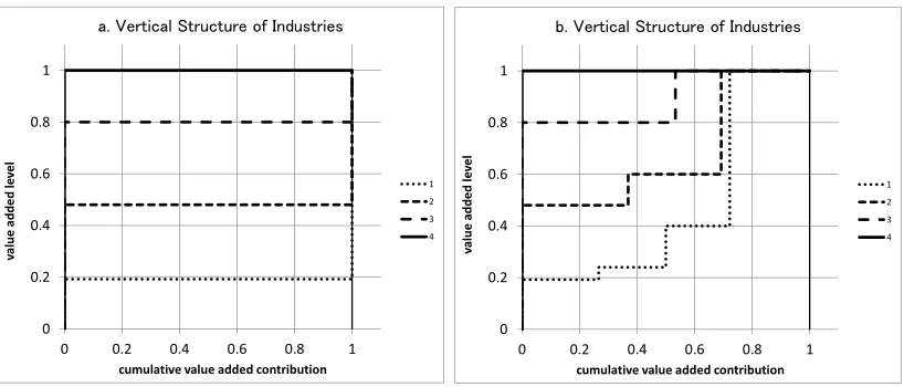
Example 1 This is a very simple example with only 4 industries. The direct requirement coefficients matrixA,

rate of value addedv, and finald demandYare given as follows:

A= ⎛ ⎜ ⎜ ⎜ ⎜ ⎜ ⎜ ⎜ ⎜ ⎜ ⎜ ⎜ ⎜ ⎜ ⎜ ⎜ ⎜ ⎜ ⎜ ⎜ ⎜ ⎜ ⎜ ⎜ ⎜ ⎜ ⎜ ⎜ ⎜ ⎜ ⎜ ⎜ ⎜ ⎜ ⎝

0 0.4 0 0

0 0 0.6 0

0 0 0 0.8

0 0 0 0

⎞ ⎟ ⎟ ⎟ ⎟ ⎟ ⎟ ⎟ ⎟ ⎟ ⎟ ⎟ ⎟ ⎟ ⎟ ⎟ ⎟ ⎟ ⎟ ⎟ ⎟ ⎟ ⎟ ⎟ ⎟ ⎟ ⎟ ⎟ ⎟ ⎟ ⎟ ⎟ ⎟ ⎟ ⎠

, v=

⎛ ⎜ ⎜ ⎜ ⎜ ⎜ ⎜ ⎜ ⎜ ⎜ ⎜ ⎜ ⎜ ⎜ ⎜ ⎜ ⎜ ⎜ ⎜ ⎜ ⎜ ⎜ ⎜ ⎜ ⎜ ⎜ ⎜ ⎜ ⎜ ⎜ ⎜ ⎜ ⎜ ⎜ ⎝ 1

0.6

0.4

0.2 ⎞ ⎟ ⎟ ⎟ ⎟ ⎟ ⎟ ⎟ ⎟ ⎟ ⎟ ⎟ ⎟ ⎟ ⎟ ⎟ ⎟ ⎟ ⎟ ⎟ ⎟ ⎟ ⎟ ⎟ ⎟ ⎟ ⎟ ⎟ ⎟ ⎟ ⎟ ⎟ ⎟ ⎟ ⎠

, Y =

⎛ ⎜ ⎜ ⎜ ⎜ ⎜ ⎜ ⎜ ⎜ ⎜ ⎜ ⎜ ⎜ ⎜ ⎜ ⎜ ⎜ ⎜ ⎜ ⎜ ⎜ ⎜ ⎜ ⎜ ⎜ ⎜ ⎜ ⎜ ⎜ ⎜ ⎜ ⎜ ⎜ ⎜ ⎝ 0 0 0 1 ⎞ ⎟ ⎟ ⎟ ⎟ ⎟ ⎟ ⎟ ⎟ ⎟ ⎟ ⎟ ⎟ ⎟ ⎟ ⎟ ⎟ ⎟ ⎟ ⎟ ⎟ ⎟ ⎟ ⎟ ⎟ ⎟ ⎟ ⎟ ⎟ ⎟ ⎟ ⎟ ⎟ ⎟ ⎠

, Y1=

⎛ ⎜ ⎜ ⎜ ⎜ ⎜ ⎜ ⎜ ⎜ ⎜ ⎜ ⎜ ⎜ ⎜ ⎜ ⎜ ⎜ ⎜ ⎜ ⎜ ⎜ ⎜ ⎜ ⎜ ⎜ ⎜ ⎜ ⎜ ⎜ ⎜ ⎜ ⎜ ⎜ ⎜ ⎝

0.2

0.4

0.7

1 ⎞ ⎟ ⎟ ⎟ ⎟ ⎟ ⎟ ⎟ ⎟ ⎟ ⎟ ⎟ ⎟ ⎟ ⎟ ⎟ ⎟ ⎟ ⎟ ⎟ ⎟ ⎟ ⎟ ⎟ ⎟ ⎟ ⎟ ⎟ ⎟ ⎟ ⎟ ⎟ ⎟ ⎟ ⎠ .

The rows and columns indicate supply and use industries respectively. As the values of matrixA’s elements show,

this economy has a very simple industry structure, particularly when final demand isY, and we can call it a vertical

linear structure. Industry 1’s product uses only its own primary resouces without receiving any intermediates,

then industry 2 use industry 1’s product as intermediate with adding its own value added, and industry 3 uses that

product as intermediate and send it forth to industry 4 with its own value added laid on it. Finally industry 4 uses

industry 3’s product as intermediate with its own value added laid on it to produce final product which is absorbed

by final demand.

Given these data, the vertical structure of industries are shown in a diagram 2-a (left). The ordinate shows

value added levels of various stages of each industry. The abscissa, correspondingly, shows cumulative value

added contributions by the same stages. In this example, the vertical structure of industries are straight, and the

industries’ hierarchical structure shown in the diagram is very simple. Industry 1 is the lowest, upstream industry,

and industry 4 is the highest, downstream industry. Industries 2 and 3 are located between them for all value added

contribution shares.

In Figure 2-b (right), the vector of final demand is changed to Y1. In this example, some portions of all

0 0.2 0.4 0.6 0.8 1

0 0.2 0.4 0.6 0.8 1

va lu e ad ded le v e l

cumulativevalueaddedcontribution

㪸㪅㩷㪭㪼㫉㫋㫀㪺㪸㫃㩷㪪㫋㫉㫌㪺㫋㫌㫉㪼㩷㫆㪽㩷㪠㫅㪻㫌㫊㫋㫉㫀㪼㫊

1 2 3 4 0 0.2 0.4 0.6 0.8 1

0 0.2 0.4 0.6 0.8 1

va lu e add ed le v e l

cumulativevalueaddedcontribution

㪹㪅㩷㪭㪼㫉㫋㫀㪺㪸㫃㩷㪪㫋㫉㫌㪺㫋㫌㫉㪼㩷㫆㪽㩷㪠㫅㪻㫌㫊㫋㫉㫀㪼㫊

1 2 3 4

Figure 2: Example 1

the order of industries’ value added levels are almost the same as the left figure. (If we change the values of final

demand vector a little, intersections of graphs will appear.)

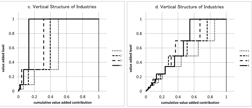
Example 2 The number of industries remains 4. In this case positions of all 4 industries are, in a sense,

sym-metrical. Industry 2 receives intermediates from industry 1, industry 3 from industry 2, industry 4 from industry

3, and industry 1 from industry 4. All of the direct requirement coefficients are the same (0.3 in the left, and 0.7 in

the right). However, final demands are biased (those of later number industries are larger than earlier ones).

A= ⎛ ⎜ ⎜ ⎜ ⎜ ⎜ ⎜ ⎜ ⎜ ⎜ ⎜ ⎜ ⎜ ⎜ ⎜ ⎜ ⎜ ⎜ ⎜ ⎜ ⎜ ⎜ ⎜ ⎜ ⎜ ⎜ ⎜ ⎜ ⎜ ⎜ ⎜ ⎜ ⎜ ⎜ ⎝

0 0.3 0 0

0 0 0.3 0

0 0 0 0.3

0.3 0 0 0

⎞ ⎟ ⎟ ⎟ ⎟ ⎟ ⎟ ⎟ ⎟ ⎟ ⎟ ⎟ ⎟ ⎟ ⎟ ⎟ ⎟ ⎟ ⎟ ⎟ ⎟ ⎟ ⎟ ⎟ ⎟ ⎟ ⎟ ⎟ ⎟ ⎟ ⎟ ⎟ ⎟ ⎟ ⎠

, A1=

⎛ ⎜ ⎜ ⎜ ⎜ ⎜ ⎜ ⎜ ⎜ ⎜ ⎜ ⎜ ⎜ ⎜ ⎜ ⎜ ⎜ ⎜ ⎜ ⎜ ⎜ ⎜ ⎜ ⎜ ⎜ ⎜ ⎜ ⎜ ⎜ ⎜ ⎜ ⎜ ⎜ ⎜ ⎝

0 0.7 0 0

0 0 0.7 0

0 0 0 0.7

0.7 0 0 0

⎞ ⎟ ⎟ ⎟ ⎟ ⎟ ⎟ ⎟ ⎟ ⎟ ⎟ ⎟ ⎟ ⎟ ⎟ ⎟ ⎟ ⎟ ⎟ ⎟ ⎟ ⎟ ⎟ ⎟ ⎟ ⎟ ⎟ ⎟ ⎟ ⎟ ⎟ ⎟ ⎟ ⎟ ⎠

, Y=

⎛ ⎜ ⎜ ⎜ ⎜ ⎜ ⎜ ⎜ ⎜ ⎜ ⎜ ⎜ ⎜ ⎜ ⎜ ⎜ ⎜ ⎜ ⎜ ⎜ ⎜ ⎜ ⎜ ⎜ ⎜ ⎜ ⎜ ⎜ ⎜ ⎜ ⎜ ⎜ ⎜ ⎜ ⎝ 1 2 3 4 ⎞ ⎟ ⎟ ⎟ ⎟ ⎟ ⎟ ⎟ ⎟ ⎟ ⎟ ⎟ ⎟ ⎟ ⎟ ⎟ ⎟ ⎟ ⎟ ⎟ ⎟ ⎟ ⎟ ⎟ ⎟ ⎟ ⎟ ⎟ ⎟ ⎟ ⎟ ⎟ ⎟ ⎟ ⎠ .

The graphs depicted on these data are shown in Figure 3-c and -d. When the direct requirement coefficient

isA(left diagram), 70 percent of all of the value added is added in the last production stage, the graphs of value

added levels jump at one step from 0.30 to 1.00. Accordingly, segments of final stage (producing final products) in

total products are large without exception. That is, the top plateau parts, which show the portions absorbed to final

demand, are relatively large for all industries (compar with the right diagram).

However, since there is a biase in final demands, quantities of final products are larger in later number

0 0.2 0.4 0.6 0.8 1

0 0.2 0.4 0.6 0.8 1

va

lu

e

ad

ded

le

v

e

l

cumulativevalueaddedcontribution

㪺㪅㩷㪭㪼㫉㫋㫀㪺㪸㫃㩷㪪㫋㫉㫌㪺㫋㫌㫉㪼㩷㫆㪽㩷㪠㫅㪻㫌㫊㫋㫉㫀㪼㫊

1 2 3 4

0 0.2 0.4 0.6 0.8 1

0 0.2 0.4 0.6 0.8 1

va

lu

e

ad

ded

le

v

e

l

cumulativevalueaddedcontribution

㪻㪅㩷㪭㪼㫉㫋㫀㪺㪸㫃㩷㪪㫋㫉㫌㪺㫋㫌㫉㪼㩷㫆㪽㩷㪠㫅㪻㫌㫊㫋㫉㫀㪼㫊

1 2 3 4

Figure 3: Example 2

level).

In the right diagram direct requirement coefficients only are changed from 0.3 to 0.7 (see the matrixA1). Thus,

value added levels are equally lower (graphs are biased towards right) relatively to the left graphs. In other words,

all industries become biased towards relatively upstream industries.

By making these graphs with actual input-output table data, we can evaluate each industries’ vertical position

in the whole economy.

Though we do not show, matrices such asA₍j) in (5) orV₍j) in (9) for industry j(=1, . . . ,4) are also easily calculated.

3

Dealing with Imports

When we are to apply our method to analyse vertical structure of industries using actual input-output tables, we

have one issue to make an adjustment for. This is how to deal with imports.

As discussed above, two factors are crucial for our analysis to evaluate an industry’s vertical position (VA

level). One is the destination industry-stages’ VA levels, to which the supply industry’s value added flows in. The

other is the amount of value added contributions by the supply industry allocated to various industry-stages in the

economy.

in use industries’ products, we should not change the evaluation of various stages’ VA levels. For, imported values

surely have contributed as an ingredient in constituting products values.

On the other hand, it is not desirable that a supply industry’s value added contribution has any imported value

whithin it. That is, we cannot use direct allocation matrix B = Xˆ−1AXˆ for evaluating supply industries’ VA

contributions.. Let us consider this further.

(i,j) element of B represents what fraction of a unit of producti is (directly) allocated to product j or use

industry j. If this economy has intermediate imports, direct requirement coefficient matrix is divided into two

parts: domestic and import direct requirement coefficient matrices, Dand M (A = D+M). Then, since B =

ˆ

X−1_{AXˆ =Xˆ}−1_DXˆ+Xˆ−1_{MXˆ, direct allocation matrixBcontains allocation of imported inputs. But imported inputs}

are supplied not by domestic industries but by foreign industries, whose value added should be excluded from

domestic industries’ contributions.

We need somewhat detailed discussion, however. SinceA=D+M, we haveX=AX+Y =DX+(MX+Y),

whereYis final demand. This final demandYis usually defined as

Y=E+EX−IM,

whereEis domestic expenditure on final products,EX exports, andIMimports. The problem is thatIM contains

both final importsFMand intermediate importsIi_M. IfYshould be to represent demand for domestic final products,

imports to be deducted fromEshould be imports of final products. But conventionally not final imports but total

(both final and intermediate) imports are deducted fromEto obtainY. In that sense,F=Y+Ii_M=E+EX−FM seems more appropriate than conventionalYas final demand per se. Let us callFgenuin final demand.

SinceIi

M=MX, we have

X=DX+(MX+Y)=DX+F.

This is solved forXas

X=(I−D)−1F=(I+D+D2+. . .)F. (13)

DenotingR=Xˆ−DXˆ andf =Xˆ−1F, we obtain

Ris different fromB, but is another allocation matrix. SinceA≥D, we also haveB≥R. Thus,I+B+B2_{+· · · ≥}

I+R+R2_{+. . ., which corresponds to and is consistent with the factY ≤F (ory≥ f). (These inequalities will}

virtually hold in the strict sense.)

In calculations with actual input-output data, we sometimes find industries whose final demand values are

negative. It is difficult to imagine what negative final demand means, and what kind of production it will induce.

But usually the cases when we have negative final demand seem ones both with large intermediate imports and

with small “genuine final demand” in the sense of our terminology,F.

In order to check this argument I examined 1998–2008 U.S. I-O annual data. In this data series, industries and

commodities are classified into 65 (excluding two ‘commodities’: 66 Scrap, and 67 Noncomparable imports). In

2008 table, for example, 5 commodities among 65 show negative “final uses” values8. But by adding intermediate

imports, all of these 5 negative values turned into positive. That is, all ofF values showed positive. The same is

true for almost all years from 1998 through 2008, except 2000 and 2002. (In these two years, ‘211 Oil and gas

extraction’ showed negative ‘genuine final demand’ values. The reason is not clear.)

Then, (14) shows proportionate allocations of domestically produced value added. In the right-hand side, the

(λ+1)-th termRλ_{f is a column vector of value added produced byndomestic supply industries that are injected}

into stage-λof various use industries. We decompose the expression (14) like C(i) in section 2.2. The matrix obtained, supply industryi’sdomestic value added (VA) contributionmatrix, is:

S(i)=

s(_{i j}λ)

= ⎛ ⎜ ⎜ ⎜ ⎜ ⎜ ⎜ ⎜ ⎜ ⎜ ⎜ ⎜ ⎜ ⎜ ⎜ ⎜ ⎜ ⎜ ⎜ ⎜ ⎜ ⎜ ⎜ ⎜ ⎜ ⎜ ⎜ ⎜ ⎜ ⎜ ⎜ ⎜ ⎜ ⎜ ⎜ ⎜ ⎜ ⎜ ⎜ ⎜ ⎜ ⎜ ⎜ ⎜ ⎜ ⎝

0 0 . . . fi . . . 0

ri1f1 ri2f2 . . . riifi . . . rinfn ..

. ... ... ... ... ...

r(_iλ₁)f1 r (λ)

i2 f2 . . . r (λ)

ii fi . . . r

(λ)

in fn .. . ... ... ... ... ... ⎞ ⎟ ⎟ ⎟ ⎟ ⎟ ⎟ ⎟ ⎟ ⎟ ⎟ ⎟ ⎟ ⎟ ⎟ ⎟ ⎟ ⎟ ⎟ ⎟ ⎟ ⎟ ⎟ ⎟ ⎟ ⎟ ⎟ ⎟ ⎟ ⎟ ⎟ ⎟ ⎟ ⎟ ⎟ ⎟ ⎟ ⎟ ⎟ ⎟ ⎟ ⎟ ⎟ ⎟ ⎟ ⎠ (15)

whererλ_{i j}is the (i,j) element ofRλ _=Xˆ−1_Dλ_{Xˆ, f}

j j-th element of vector f, ands

(λ)

i j =r λ

i jfj. We have to use this

S(i) to evaluate domestic supply industries’ VA contributions.

Next issue to be considered is the value added contribution by imports. As discussed above, the height of VA

8_{These are 2. Forestry, fishing, and related activities, 3. Oil and gas extraction, 8. Wood products, 9. Nonmetallic mineral products, and 10.}

levels to which imported intermediates flow in is not affected by existence of imports, except an issue discussed

shortly.

On the other hand, value added contributions by imports have some crucial points to be considered. First total

productionXis shown as (13). Then intermediate imports vector is:

MX=M(I+D+D2+. . .)F.

(This does not contain final good imports.) Obviously, this is directly required imports to produce total outputX,

not containing ‘indirect’ imports. for there is no such thing as ‘indirect’ import. If some product is imported, its

earlier production stages are basically carried in foreign countries, and earlier stages does not have any effect on

this country’s inputs requirement9.

But this discussion evokes one probably important point. When a country imports a product, it brings into this

country not only value added of its final production stage but also all the value added created and piled in all the

previous stages.

This has something in relation to the value added levels mentioned above. As shown in (2),u′_=u′_A+

v′. That

is, each product’s value is equal to its intermediates’ value plus value added created by the use industry. Dividing

AintoDandM, we obtain

u′=u′(D+M)+v′.

From this equation, the following expression is obtained:

u′=u′M(I−D)−1+v′(I−D)−1

=u′M(I+D+D2+· · ·)+v′(I+D+D2+· · ·). (16) The first termu′M(I+D+D2+· · ·_{) of the right-hand side is the value of intermediate imports that are necessary}

to produce one units of each domestic product. What is important is that the amounts are expressed in product

value, not value added. The second termv′(I+D+D2_{+· · ·) is the amount of value added as recognized asv}′

is multiplied. In other words, though the term does not containv′,u′_M

(I+D+D2_{+· · ·) isthevalue added that}

imports contribute in forming a unit value of each product.

9_{This statement does not hold, if some of foreign countries which export to this country use imported intermediates from this country in}

This can be shown in a somewhat different way. (3) shows each industry product’s value added composition.

Since this is equal to (16), we have

u′M(I+D+D2+· · ·)=v′(I+A+A2+· · ·)−v′(I+D+D2+· · ·).

The difference between total value added (first term) and domestically produced value added (second term), that

is, value added injected by imported products, is equal tou′_M

(I+D+D2_{+· · ·).}

This is a point we should keep in mind when we want to evaluate the contribution of imports in VA level

formation.

4

Some Emprical Application

In this section we make an attempt to apply our method to actual input-output data. We pick up 1998–2008 annual

I-O Tables constructed by U.S. Bureau of Economic Analysis10. These tables consist of 65 industries and 67

commodities (including “66 Scrap, used and second hand goods” and “67 Non-comparable imports and

rest-of-the-world adjustment)11_{. When we want to analyse individual industries relatively in detail, finer classification of}

industries is desirable. U.S. Benchmark detailed tables are released every some 5 years and have more than 400

industries classified, but its industry (commodity) classificatin system has been changed by Benchmark years. That

makes it difficult to compare different years.

One point we need to discuss and have yet to do is U.S. I-O tables are produced by the

commodity-by-industry approach. There have been raised a lot of problems and discussions in the literature about how to produce

commodity-by-commodity or industry-by-industry tables from these original commodity-by-industry tables12_{. We}

used U.S. annual tables of “After Redefinition”, where redefining procedures have made the concept of industries

much clearer than original tables. U.S. B.E.A. also provide three kinds of tables: 1. Commodity-by-commodigy

(CxC) total requirements (coefficients) tables, 2. industry-by-industry (IxI) total requirements (coefficients) tables,

and 3. Industry-by-commodity (IxC) total requirements (coefficients) tables.

10_{U.S. Bureau of Economic Analysis [1]. This file (a set of several files) is downloadable from BEA’s website.}

11_{We could use OECD input-output tables. If we used OECD tables, we could compare different countries’ vertical structures of industries.}

But, OECD tables are composed of somewhat small numbers of industries (commodities). OECD tables are also downloaded from its website.

See also N. Yamano and N. Ahmad [8] and Wixted, B., N. Yamano and C. Webb, [7].

For analytical purposes, it is more convinient to use tables with formats of commodity-by-commodity or

industry-or-industry. In order to transform data (data vectors and matrices) from one format to the other, we

need a transformatin matrixW which transforms commodity vector to industry vector. Fortunately, this can be

obtained by calculating with total requirements tables produced in the two (CxC and IxI) formats. The direct

method to calculate transformation matrixWis explained in Chapter 12 of Karen J. Horowitz and Mark A.

Plant-ing [3] (so-called US I-O manual). But we obtained the transformation by calculatPlant-ing in reverse order, that is, by

deduction from completed CxC and IxI tables.

In the original tables, values of final demands are given in commodity units. This is a reason why our

calcula-tion is carried out basically on CxC tables.

Average VA contribution levels First, we calculated average VA contribution levels of (supply) industries. The

larger and closer to 1 the contribution level calculated is, the more closely positioned to final demand is the industry.

In other words, industries with higher VA contribution levels are relatively ‘downstream’ industries. Those with

lower VA contribution levels are relatively ‘upstream’ ones.

Average VA contribution levels of 65 industries (shown by commodity base) are calculated. The results are

shown in Appendix A, “Average VA contribution levels of U.S. Industries”. Industries (commodities) are sorted

rearranged by 2008 contribution levels in ascending order. Industries placed in upper part of the table are relatively

‘upstream’ industries, and those in lower part relatively ‘downstream’ industries.

Graphs of VA contribution levels Next, we tried to show VA contribution level structure of each (supply)

industry by depicting graphs according to the method explained in 2.3. Our procedure of calculations is as follows.

(Our calculation of power matrix series was carried up to 10th power, which is apparently enough.)

First we calculated value added levels of industries. This calculation was based on (4),h′

(λ)=u′_Aλ_.

Calcu-lation results were rearrannged by each supply industryito obtain matrices ofA(i)’s. Then, we calculated value added contribution segments of supply industries to get the VA level matrixL, which was rearranged again in VA level’s ascending order. Finally cumulative value added contribution shares were calculated. Then value added

level and value added contribution shares of each supply industry-stage were paired to depict graphs. Of course,

Obtained 65 U.S. industry graphs (commodity-base) are shown in the Appendix A. Each industry has three

(kinked) curves for years 1998, 2003, and 2008. All curves in the graphs start from origin and reach (1.1). But

there are little which move along the diagonal. Some curves are biased towards lower right, and others towards

upper left.

In general, industries whose curves are biased towards lower left may be called upstream industries. These

inclulde 211. Oil and gas extraction, 331. Primary metals, 323. Printing and related support activities, and so on.

5412OP Mioscellaneous professional, scientific, and technical services is included in this category too.

On the other hand, industries whose curves are biased towards upper left can be called downstream industries.

Many industries are in this category. They tend to have larger segments of stage-0 (final demand) in total product

allocation. But we should be cautious about looking at the segments of final demand. That is, the two main

cate-gories of final demand are consumption and investment. Though investment is conventionally and for convinience

classified as final demand, it can be regarded as intermediate in the longer roundabout prouction processes. 213.

Support activities for mining and 333. Machinery are probably its typical cases. Large parts of their products are

absorbed into investments, which makes their average VA contribution levels high or their graphs biased towards

upper left, it might not match our common sense.

Making these graphs are, of course, only one step towards vertical structure analysis of industries. If we want

to analyse relationships between individual industries, we need an analysis peculiar to that relationship. But even

in that case, knowing what is individual industrys’ vertical position in the whole economy will be helpful and

sometimes indispensable.

5

Concluding Remarks

The main purpose of this paper is to propose a method to analyse vertical structure of industries. When our attempt

of this kind is to show industries’ positions in the whole economy, analysis based on input-output data seems

inevitable.

Our method of analysis, particularly the one displayed by graphs of value added contribution levels, is, in a

sense, an integration of quantity model and price model of input-output tables. The concept of value added level

contributions is derived from the quantity aspect, on the other.

In this context,proper dealing with imports seems very important, as discussed earlier. Value added brought

in by imports are not created in this country. But accurate domestic direct requirements tables cannot obtained

without accurate import requirements tables. Unfortunately, usually (competitive) import data are not gathered

separately from domestic data. Import requirements matrix is constructed with several approximation methods. I

do not know how import requirements data are accurate or inaccurate, but I wonder a lot of analitical possibilites in

this field might be lost for this reason. Even so, the method shown here may, we hope, have some value to advance

References

[1] Bureau of Economic Analysis, U.S. Department of Commerce. 1998-2008 Annual I-O Tables. U.S. Bureau

of Economic Analysis’s website:http://www.bea.gov/industry/io_annual.htm, 2010.

[2] Jiemin Guo, Ann M. Lawson, and Mark A. Planting. From Make-Use to Symmetric I-O Tables: An

As-sessment of Alternative Technology Assumptions. Paper presented at the 14th International Conference on

Input-Output Techniques, October 10-15, 2002, Montreal, Canada, October 10-15 2002.

[3] Karen J. Horowitz and Mark A. Planting. Concepts and Methods of the Input-Output Accounts. website of

U.S. Bureau of Economic Analysis of the U.S. Department of Commerce, September 2006.

[4] David Hummels, Jun Ishii, and Kei-Mu Yi. The Nature and Growth of Vertical Specialization in World Trade.

Journal of International Economics, Vol. 54, pp. 75–96, 2001.

[5] Ronald E. Miller and Peter D. Blair. Input-Output Analysis: Foundations and Extentions. Cambridge Univ.

Pr., Cambridge U.K., 2nd ed. edition, 2009.

[6] UNCTAD. The Offshoring of Corporate Service Functions: The Next Global Shift?, chapter 4, pp. 147–80.

2004.

[7] B. Wixted, N. Yamano, and C. Webb. Input-Output Analysis in an Increasingly Globalised World:

Applica-tions.OECD Science, Technology and Industry Working Papers, Vol. 2006/7, .

[8] N. Yamano and N. Ahmad. The OECD Input-Output Database: 2006 Edition. OECD Science, Technology

Appendix A.

Average VA contribution levels of US industries

code commodity 1998 2003 2008

1 493 Warehousing and storage 0.3278 0.3206 0.3460

2 561 Administrative and support services 0.3462 0.3511 0.3599

3 211 Oil and gas extraction 0.3350 0.3368 0.3713

4 323 Printing and related support activities 0.3386 0.3367 0.3745

5 GFE Federal government enterprises 0.3930 0.3686 0.3790

6 486 Pipeline transportation 0.3297 0.3691 0.3955

7 5412OP Miscellaneous professional, scientific, and technical services 0.3991 0.3929 0.4133

8 113FF Forestry, fishing, and related activities 0.3913 0.4063 0.4187

9 321 Wood products 0.5082 0.4503 0.4346

10 562 Waste management and remediation services 0.4251 0.4262 0.4396

11 55 Management of companies and enterprises 0.4355 0.4528 0.4778

12 487OS Other transportation and support activities 0.4306 0.4343 0.4816

13 212 Mining, except oil and gas 0.4067 0.3871 0.4840

14 331 Primary metals 0.4494 0.4437 0.4878

15 521CI Federal Reserve banks, credit intermediation, and related activities 0.5382 0.4877 0.4878

16 327 Nonmetallic mineral products 0.5011 0.4739 0.4937

17 332 Fabricated metal products 0.5030 0.5013 0.5074

18 322 Paper products 0.4550 0.4780 0.5151

19 326 Plastics and rubber products 0.5162 0.5050 0.5285

20 482 Rail transportation 0.5085 0.5091 0.5467

21 514 Other information services 0.4057 0.5278 0.5546

22 5411 Legal services 0.5636 0.5650 0.5808

23 532RL Rental and leasing services and lessors of intangible assets 0.5949 0.5798 0.6100

24 524 Insurance carriers and related activities 0.6194 0.6178 0.6128

25 324 Petroleum and coal products 0.5926 0.5905 0.6151

26 512 Motion picture and sound recording industries 0.5944 0.6258 0.6219

27 325 Chemical products 0.5817 0.6215 0.6222

28 711AS Performing arts, spectator sports, museums, and related activities 0.6263 0.6126 0.6226

29 523 Securities, commodity contracts, and investments 0.6147 0.5543 0.6444

30 513 Broadcasting (except internet) and telecommunications 0.6066 0.6224 0.6466

31 111CA Farms 0.6242 0.6231 0.6517

32 22 Utilities 0.6348 0.6416 0.6594

33 484 Truck transportation 0.6281 0.6277 0.6626

34 313TT Textile mills and textile product mills 0.6120 0.6892 0.7166

35 5415 Computer systems design and related services 0.7435 0.7332 0.7235

36 42 Wholesale trade 0.7116 0.7279 0.7322

37 721 Accommodation 0.7265 0.7283 0.7343

38 485 Transit and ground passenger transportation 0.6782 0.7017 0.7365

39 335 Electrical equipment, appliances, and components 0.6918 0.7277 0.7387

40 531 Real estate 0.8072 0.7931 0.7786

41 81 Other services, except government 0.7586 0.7945 0.8014

42 339 Miscellaneous manufacturing 0.7666 0.8025 0.8016

43 481 Air transportation 0.7630 0.7570 0.8056

44 334 Computer and electronic products 0.7889 0.8110 0.8093

45 311FT Food and beverage and tobacco products 0.7940 0.7985 0.8143

46 337 Furniture and related products 0.8683 0.8366 0.8199

47 3364OT Other transportation equipment 0.8142 0.8291 0.8425

48 GSLE State and local government enterprises 0.8398 0.8428 0.8448

Average VA contribution levels of US industries---continued

50 511 Publishing industries (includes software) and internet broadcasting 0.8108 0.8596 0.8565

51 333 Machinery 0.8347 0.8410 0.8594

52 3361MV Motor vehicles, bodies and trailers, and parts 0.8338 0.8397 0.8595

53 722 Food services and drinking places 0.8589 0.8504 0.8617

54 23 Construction 0.9031 0.8964 0.9002

55 483 Water transportation 0.8345 0.8859 0.9364

56 44RT Retail trade 0.9409 0.9392 0.9486

57 525 Funds, trusts, and other financial vehicles 0.9674 0.9433 0.9516

58 713 Amusements, gambling, and recreation industries 0.9784 0.9410 0.9517

59 61 Educational services 0.8893 0.9373 0.9531

60 213 Support activities for mining 0.9232 0.9281 0.9641

61 621 Ambulatory health care services 0.9678 0.9748 0.9758

62 624 Social assistance 0.9633 0.9885 0.9943

63 622HO Hospitals and nursing and residential care facilities 0.9923 0.9957 0.9979

64 GFG Federal general government 1.0000 1.0000 1.0000

65 GSLG State and local general government 1.0000 1.0000 1.0000

Appendix B. Vertical Structure of U.S. Industries (commodity base) for 1998, 2003 and 2008

5

10

15

335 Electrical equipment, appliances, and components

3361MV Motor vehicles, bodies and trailers, and parts

332 Fabricated metal products 333 Machinery 334 Computer and electronic products

212 Mining, except oil and gas 213 Support activities for mining

22 Utilities 23 Construction 321 Wood products 327 Nonmetallic mineral products 331 Primary metals

111CA Farms 113FF Forestry, fishing, and related activities 211 Oil and gas extraction

0 0.2 0.4 0.6 0.8 1 1.2

0 0.2 0.4 0.6 0.8 1 1.2 1.4

Y1998 Y2003 Y2008 0 0.2 0.4 0.6 0.8 1 1.2

0 0.2 0.4 0.6 0.8 1 1.2

Y1998 Y2003 Y2008 0 0.2 0.4 0.6 0.8 1 1.2

0 0.2 0.4 0.6 0.8 1 1.2

Y1998 Y2003 Y2008 0 0.2 0.4 0.6 0.8 1 1.2

0 0.2 0.4 0.6 0.8 1 1.2

Y1998 Y2003 Y2008 0 0.2 0.4 0.6 0.8 1 1.2

0 0.2 0.4 0.6 0.8 1 1.2

Y1998 Y2003 Y2008 0 0.2 0.4 0.6 0.8 1 1.2

0 0.2 0.4 0.6 0.8 1 1.2

Y1998 Y2003 Y2008 0 0.2 0.4 0.6 0.8 1 1.2

0 0.2 0.4 0.6 0.8 1 1.2

Y1998 Y2003 Y2008 0 0.2 0.4 0.6 0.8 1 1.2

0 0.2 0.4 0.6 0.8 1 1.2

Y1998 Y2003 Y2008 0 0.2 0.4 0.6 0.8 1 1.2

0 0.2 0.4 0.6 0.8 1 1.2

Y1998 Y2003 Y2008 0 0.2 0.4 0.6 0.8 1 1.2

0 0.2 0.4 0.6 0.8 1 1.2

Y1998 Y2003 Y2008 0 0.2 0.4 0.6 0.8 1 1.2

0 0.2 0.4 0.6 0.8 1 1.2

Y1998 Y2003 Y2008 0 0.2 0.4 0.6 0.8 1 1.2

0 0.2 0.4 0.6 0.8 1 1.2

Y1998 Y2003 Y2008 0 0.2 0.4 0.6 0.8 1 1.2

‐0.2 0 0.2 0.4 0.6 0.8 1 1.2

Y1998 Y2003 Y2008 0 0.2 0.4 0.6 0.8 1 1.2

0 0.20.40.60.8 1 1.21.4

Y1998 Y2003 Y2008 0 0.2 0.4 0.6 0.8 1 1.2

0 0.2 0.4 0.6 0.8 1 1.2

Y1998

Y2003

Vertical Structure of U.S. Industries (commodity base) ---continued

20

25

30

324 Petroleum and coal products 325 Chemical products 3364OT Other transportation equipment 337 Furniture and related products 339 Miscellaneous manufacturing 311FT Food and beverage and tobacco products 313TT Textile mills and textile product mills

315AL Apparel and leather and allied products 322 Paper products 323 Printing and related support activities

481 Air transportation 482 Rail transportation 326 Plastics and rubber products 42 Wholesale trade 44RT Retail trade

0 0.2 0.4 0.6 0.8 1 1.2

0 0.2 0.4 0.6 0.8 1 1.2

Y1998 Y2003 Y2008 0 0.2 0.4 0.6 0.8 1 1.2

0 0.2 0.4 0.6 0.8 1 1.2

Y1998 Y2003 Y2008 0 0.2 0.4 0.6 0.8 1 1.2

0 0.2 0.4 0.6 0.8 1 1.2

Y1998 Y2003 Y2008 0 0.2 0.4 0.6 0.8 1 1.2

0 0.2 0.4 0.6 0.8 1 1.2

Y1998 Y2003 Y2008 0 0.2 0.4 0.6 0.8 1 1.2

0 0.2 0.4 0.6 0.8 1 1.2

Y1998 Y2003 Y2008 0 0.2 0.4 0.6 0.8 1 1.2

0 0.2 0.4 0.6 0.8 1 1.2

Y1998 Y2003 Y2008 0 0.2 0.4 0.6 0.8 1 1.2

0 0.2 0.4 0.6 0.8 1 1.2

Y1998 Y2003 Y2008 0 0.2 0.4 0.6 0.8 1 1.2

0 0.2 0.4 0.6 0.8 1 1.2

Y1998 Y2003 Y2008 0 0.2 0.4 0.6 0.8 1 1.2

0 0.2 0.4 0.6 0.8 1 1.2

Y1998 Y2003 Y2008 0 0.2 0.4 0.6 0.8 1 1.2

0 0.2 0.4 0.6 0.8 1 1.2

Y1998 Y2003 Y2008 0 0.2 0.4 0.6 0.8 1 1.2

0 0.2 0.4 0.6 0.8 1 1.2

Y1998 Y2003 Y2008 0 0.2 0.4 0.6 0.8 1 1.2

0 0.2 0.4 0.6 0.8 1 1.2

Y1998 Y2003 Y2008 0 0.2 0.4 0.6 0.8 1 1.2

0 0.2 0.4 0.6 0.8 1 1.2

Y1998 Y2003 Y2008 0 0.2 0.4 0.6 0.8 1 1.2

0 0.2 0.4 0.6 0.8 1 1.2

Y1998 Y2003 Y2008 0 0.2 0.4 0.6 0.8 1 1.2

0 0.2 0.4 0.6 0.8 1 1.2

Y1998

Y2003

Vertical Structure of U.S. Industries (commodity base) ---continued

35

40

45

513 Broadcasting (except internet) and

telecommunications 514 Other information services 483 Water transportation 484 Truck transportation 485 Transit and ground passenger

transportation 486 Pipeline transportation

487OS Other transportation and support activities

493 Warehousing and storage 511 Publishing industries (includes software) and internet broadcasting

512 Motion picture and sound recording industries

521CI Federal Reserve banks, credit intermediation, and related activities

523 Securities, commodity contracts, and

investments 524 Insurance carriers and related activities 525 Funds, trusts, and other financial vehicles 531 Real estate 0 0.2 0.4 0.6 0.8 1 1.2

0 0.2 0.4 0.6 0.8 1 1.2

Y1998 Y2003 Y2008 0 0.2 0.4 0.6 0.8 1 1.2

0 0.2 0.4 0.6 0.8 1 1.2

Y1998 Y2003 Y2008 0 0.2 0.4 0.6 0.8 1 1.2

0 0.2 0.4 0.6 0.8 1 1.2

Y1998 Y2003 Y2008 0 0.2 0.4 0.6 0.8 1 1.2

0 0.2 0.4 0.6 0.8 1 1.2

Y1998 Y2003 Y2008 0 0.2 0.4 0.6 0.8 1 1.2

0 0.2 0.4 0.6 0.8 1 1.2

Y1998 Y2003 Y2008 0 0.2 0.4 0.6 0.8 1 1.2

0 0.2 0.4 0.6 0.8 1 1.2

Y1998 Y2003 Y2008 0 0.2 0.4 0.6 0.8 1 1.2

0 0.2 0.4 0.6 0.8 1 1.2

Y1998 Y2003 Y2008 0 0.2 0.4 0.6 0.8 1 1.2

0 0.2 0.4 0.6 0.8 1 1.2

Y1998 Y2003 Y2008 0 0.2 0.4 0.6 0.8 1 1.2

0 0.2 0.4 0.6 0.8 1 1.2

Y1998 Y2003 Y2008 0 0.2 0.4 0.6 0.8 1 1.2

0 0.2 0.4 0.6 0.8 1 1.2

Y1998 Y2003 Y2008 0 0.2 0.4 0.6 0.8 1 1.2

0 0.2 0.4 0.6 0.8 1 1.2

Y1998 Y2003 Y2008 0 0.2 0.4 0.6 0.8 1 1.2

0 0.2 0.4 0.6 0.8 1 1.2

Y1998 Y2003 Y2008 0 0.2 0.4 0.6 0.8 1 1.2

0 0.2 0.4 0.6 0.8 1 1.2

Y1998 Y2003 Y2008 0 0.2 0.4 0.6 0.8 1 1.2

0 0.2 0.4 0.6 0.8 1 1.2

Y1998 Y2003 Y2008 0 0.2 0.4 0.6 0.8 1 1.2

0 0.2 0.4 0.6 0.8 1 1.2

Y1998

Y2003