Higher order volatility: time series

Munich Personal RePEc Archive

Higher-order volatility: time series

Carey, Alexander

12 January 2010

Online at

https://mpra.ub.uni-muenchen.de/21087/

Page 1 of 35

HIGHER-ORDER VOLATILITY: TIME SERIES

Alexander Carey

6 rue de l’Abbé Groult 75015 Paris, France [email protected]

January 12, 2010

This paper presents time-series of higher-order volatilities for the S&P 500 and EURUSD. We use a 3-volatility model which accounts for non-normal skewness and kurtosis. The volatilities control the level, slope and curvature of the Black-Scholes implied volatility smile; accordingly we term them "base", "skew" and "smile" volatility. We define instantaneous skewness and kurtosis as simple ratios of the volatilities, and show that when these metrics are held constant, the model is relative sticky-delta.

For the S&P 500 in 2008, skew and smile volatility are highly correlated with base volatility. Instantaneous skewness and kurtosis are remarkably stable, including over the market dislocation of the last four months of the year. Daily changes in all three volatilities are correlated with daily returns. For EURUSD in 2006, base and smile volatility are closely correlated, but in contrast to the equity case, skew volatility is independent and changes sign. This change in sign appears to provide advance warning of the two major market moves of the year. However, daily changes in the volatilities are uncorrelated with daily returns.

1. THE MODEL

1.1 Basic definitions and results

Here we recall some basic definitions and results from Carey (2005, 2006). Let

X

_t

( )

be a positive-valued adapted stochastic process on a filtered probability space

!

,

F

,

F

t

( )

,

Q

(

)

,

t

_!

0

_{, satisfying the usual conditions. Here}

X

t

( )

is interpreted as the market price of a financial security,

( )

F

_t as the market information structure, and

Q

as an equivalent martingale measure. Let

!t

_>

0

_{denote a finite period of time, and define}

!

X

t

=

X

t₊!t

"

X

t, so that the security return over the interval

t

to

t

+

!

t

reads

!

X

t

X

t .

E

t

!

Page 2 of 35

We define

j

-th order finite-period volatility

_!

_j,t via the identity:

!

j,t j

_"

E

_t

#

_X

t

X

t

(

)

j

#

_t

_,

with the convention that

_!

_j,t equals the non-negative root when

j

is even, and we let

!

j,t

=

lim

"t!0

#

j,t denote

j

-th order instantaneous volatility. In Carey (2005) a simple

thought experiment shows how to interpret

_!

_j,t and its limit

!

j,t as standard changes.

Mathematically, the quantities

!

j,t

X

t

(

)

j

,

j

₌

1, 2,...

can be characterised as infinitesimal

moments. They are defined in Gikhman and Skorokhod (1972) in the context of Markov

processes, and have begun to appear in the finance literature — see e.g. Johannes (2004).

We assume that the security has market-independent returns under the equivalent martingale measure

Q

. We define this to mean that for any

t

_and

!

t

, the security return

!

X

t

X

t is independent of

F

t, the information available to investors at

time

t

_{. If the information available to investors is limited to that represented by the}

security price history, or if all extraneous information is irrelevant to investors, this reduces to the more common assumption of independent (relative) increments.1 _{It also}

implies that the instantaneous volatility processes

!

j,t

,

j

=

1, 2,...

are deterministic. We

make the further assumption that over arbitrarily small intervals of time, the security almost surely does not double in price.

Under these premises, the characteristic function of the log return

_ln

X

_t

+!

X

t

(

)

reads:

!(")

=

exp

i

"

j

#

$%

&

'(

)

j,u j

du

t t+*

+

j=1

,

-

,

with

!

1,t

=

b

t, the instantaneous cost of carry of the security. See Appendix 1 for a

derivation. This formula and a related one were originally obtained in Carey (2005, 2006) under the assumption that the finite-period volatilities are deterministic for very small time horizons

!t

. While not as clean as the assumption we make above, it perhaps carries more intuition. When higher-order volatilities are zero, this characteristic function reduces to that of the Black and Scholes (1973) and Merton (1973) model.

The market price

C

_{of a European-exercise, path-independent option satisfies the}

partial differential equation (PDE):

!

_t

C(

X,t)

₊

1

j!

"

j,t j

X

j

!

_Xj

C(X,

t)

j=1 #

$

=

r

t

C(

X,

t)

,

where

r

t is the riskless rate of interest at time

t

. This can be viewed as an infinite-order

version of the (second-order) Black-Scholes PDE. As indicated, the sequence of volatilities

!

j,

j

=

1, 2,...

can be truncated at

j

=

2

to yield the Black-Scholes model. It

cannot however be truncated at any higher order, and must remain infinite.2

1

Often the market information structure is exogeously limited to the security price history, albeit implicitly (and perhaps, sometimes, unwittingly). There is however no good basis for this assumption, as pointed out by e.g. Babbs ans Selby (1998) and Brody et al (2007).

2

Page 3 of 35 We define the average volatility

!

j via:

!

_jj

_"

1

#

!

j,u

j

_du

t t+#

$

,

again with the convention that

!

j be non-negative when

j

is even. The (Fisher)

skewness and kurtosis of a random variable are given by:

!

1

=

c

₃

c

₂3 2 ,

!

2

=

c

4

c

2 2

where

c

j is the j-th central cumulant — see e.g. Abramowitz and Stegun (1972), p.928.

It can be shown that when all infinitesimal moments of a stochastic process exist, so do the infinitesimal cumulants, and further that the two sequences are identically equal (see Appendix 2). It follows that, to first order in

!

t

:

c

_j

₌

!

j j

_"

t

,

j

₌

1, 2...

and the skewness and kurtosis corresponding to this approximation read:

!

1

=

"

3,t

"

2,t

#

$%

&

'(

3

1

)

t

,

!

₂

₌

"

4,t

"

2,t

#

$%

&

'(

4

1

)

t

. (1)

These quantities are not standardised for time, and become infinite as

!t

tends to zero. This is not a reflection of any misbehaving on the part of the stochastic process, but rather that these coefficients were not designed for this setting. We therefore suggest defining instantaneous skewness

!t

and instantaneous kurtosis

_!

t as:

!

t

=

"

3,t

"

2,t

,

!

_t

₌

"

4,t

"

2,t

where the exponents in (1), serving no purpose, have been dropped. Note that these coefficients are defined for any stochastic process for which they exist, and not simply for a process with

F

_t-independent increments. We further define average instantaneous

skewness and kurtosis as:

!

=

"

3

"

2

,

!

₌

"

4

"

2

.

This is something of a misnomer, because

! "

!u

du

t t₊#

$

and

! "

!

u

du

t

t₊#

$

in general. However, it is always the case that

!t

₌

lim

" #t

!

and

!

t

=

lim

" #t

!

. The quantities

!

,

"

will

Page 4 of 35

1.2 The reduced Merton jump-diffusion implementation

Here we make use of the Merton (1976) jump-diffusion model to obtain a pricing formula that depends on the volatilities of order 2, 3 and 4. The full Merton model with lognormal jumps has four free risk parameters: the volatility

!

, the jump rate

!

, the jump size mean

!

and its standard deviation

!

. We only require three free parameters, and so reduce the parameter set by exogenously setting

!

_T

₌

₁

. This choice is motivated both by the analytical simplification that results, and by the empirical behaviour of the marked-implied

!

which, in the equity index setting at least, tends to decrease as time to expiration increases (see Carey (2005)).

The option pricing formula then simplifies to:

BSM

_n

n

!

n₌0

!

"

where

BSM

n is the Black-Scholes-Merton formula with cost of carry and volatility given

by:

b

n

=

b

+

n

_{! "}

m

1

T

,

v

n

=

!

2

+

n

"

2

T

respectively. As noted in Carey (2005), we do not assume that the risk-neutral process is a Merton lognormal jump-diffusion (with or without

!

_T

₌

₁

); the formula is simply borrowed for reasons of analytical tractability.

A general formula giving

j

-th order volatility in terms of the Merton jump-diffusion parameters can be found in Carey (2005). With this formula,

j

-th order volatility is readily computed from the jump-diffusion parameters. However, because the formula is highly nonlinear, obtaining the jump-diffusion parameters from a set of volatilities is more involved. Under the simplification set out above, the parameter equations reduce to:

!

2

2

_T

₌

_!

2

_T

₊

_A

2

_B

_"

₂

_A

₊

₁

_,

!

₃3

_T

₌

_A

3

_B

3

"

3

_A

2

_B

₊

3

_A

"

1

_,

!

₄4

_T

₌

_A

4

_B

6

"

4

_A

3

_B

3

₊

6

_A

2

_B

"

4

_A

₊

1

subject to the constraints

_A

_>

0

_,

_B

_!

₁

_{, where}

A

₌

e

!

,

B

₌

e

"2_{. The last two equations can}

be solved analytically for

_A

,

_B

using symbolic mathematics software (we use MuPad, packaged with Matlab). The first equation then yields

!

.

In this way, we obtain an option pricing formula that depends on the three risk parameters

!

₂

"

!

₃

"

!

₄. However, this formula can be somewhat unstable, because there are many combinations of these three parameters that are not admissible. A combination of parameters that is admissible can abruptly become inadmissible under a small change in one of the parameters. In the next section we will see evidence that the ratios

!

=

"

3

"

2 and

!

=

"

₄

"

₂, defined above as average skewness and kurtosis, are

substantially more stable over time than their respective numerators. It will be useful then to consider the alternative parameter interface

!

₂

"

# " $

, in which

!

2 can be varied

over a wide range without leaving the domain of the pricing formula.

Below is an example of a volatility surface with constant volatilities. The volatilities chosen here correspond to typical values found in S&P 500 options market in the course of the year 2008, at roughly the 3-month expiration mark. The input volatilities are

!

Page 5 of 35

parameters are

!

₌

8.68%, (

"

₌

4),

#

₌

$

5.91%,

%

₌

8.81%

. The spot underlying is 100, and both the cost of carry and the rate of interest are zero.

Figure 1

Example volatility surface

The input volatilities are

!

2

=

22%,

!

3

=

"

17%,

!

4

=

18%

. The spot and forward prices both equal 100 units.

1.3 Volatility smile dynamics and price sensitivities

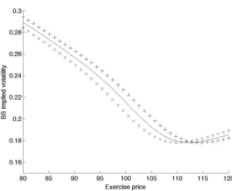
First we examine the behaviour of the volatility smile under changes in the spot price of the underlying security. In figure 2, the spot price is increased and decreased by a small amount. Evidently, the volatility smile shifts right and left respectively, that is, the smile follows the spot price. This behaviour is known as sticky moneyness (see e.g. Daglish et al (2007)), and is a hallmark of jump-diffusion/Lévy processes.

[image:7.595.122.458.162.438.2]

Page 6 of 35

Figure 2

The Black-Scholes implied volatility smile under changes in spot price

The solid line is the initial volatility smile. The pluses (crosses) are the volatility smile resulting from an increase (decrease) of 2 units in the underlying security price. The initial spot price is 100 units. Volatilities remain constant.

With fourth-order volatility (labelled HOV[4]), we notice from figure 3 that the implied volatility smile curvature increases (decreases) as

!

4 increases (decreases);

thus

!

4 predominantly affects the smile shape in implied volatilities. This is confirmed by

the graph of option price sensitivities to

!

4 in figure 4. An increase in magnitude mildly

increases the price of away-from-the-money options, but sharply lowers the prices of at-the-money options. We shall term

!

4 smile volatility.

Turning now to second-volatility, we see in figure 3 (labelled HOV[2]) that its influence on the implied volatility smile is more clear-cut: unlike with skew or smile volatility, an increase (decrease) increases (decreases) implied volatilities across all exercise prices. This effect is most pronounced in a region some way to the right of the spot price. Indeed the option price sensitivity to

!

2, plotted in figure 4, is positive

[image:8.595.102.489.180.493.2]

Page 7 of 35

Figure 3

Black-Scholes implied volatility smile sensitivities to higher-order volatilities

The solid line is the initial volatility smile. The pluses (crosses) are the volatility smile resulting from an increase (decrease) of 0.01 in higher-order volatility. The spot underlying is at 100.

The above analysis holds under the

!

₂

"

!

₃

"

!

₄ parameterisation, and each volatility was varied in turn while holding the others constant. Under the alternative

!

₂

"

# " $

parameterisation, introduced in subsection 1.2, the picture for the last two parameters of the interface is very similar. Indeed, varying the skewness metric

!

=

"

3

"

2 by itself is the same as varying skew volatility

!

3 independently of the other

two volatilities, and likewise varying the kurtosis

!

₌

"

4

"

2 by itself is the same as varying smile volatility

!

[image:9.595.100.491.166.484.2]

Page 8 of 35

Figure 4

Call or put option price sensitivities to higher-order volatilities

However, varying second-order volatility

!

2 in the

!

2

"

# " $

interface has a

different result than in the

!

₂

"

!

₃

"

!

₄ interface. The plot in figure 3 labelled “CONSTANT RATIOS” shows that an increase (decrease) in

!

2, while holding skewness

!

and

kurtosis

_!

constant, results in a parallel shift upwards (downwards) of the entire implied volatility curve. The corresponding option price sensitivities are shown in figure 4, with a positive-valued bell-shaped curve that is somewhat wider and flatter than for the

[image:10.595.127.459.191.463.2]

Page 9 of 35

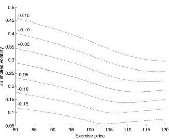
Figure 5

Black-Scholes implied volatility smile sensitivity to base volatility in the

!

₂

"

# " $

parameterisation

The solid line is the initial volatility smile. The spot underlying is at 100.

In fact, this pattern extends over a surprisingly wide interval around the original

!

2. Figure 5 shows the result of increasing (decreasing)

!

2 at intervals of 5%. Again we

see almost perfectly parallel shifts in implied volatilities. Together with the sticky-moneyness nature of the model, in which the implied volatility curve shifts left or right with the spot price, the sensitivity with respect to

!

2 within the

!

2

"

# " $

parameterisation is strongly consistent with the application of the popular trader’s rule known as “relative sticky moneyness,” in which the volatility curve shifts both sideways with the spot price, and up and down with ATM volatility — see Daglish et al (2007). We shall refer to

!

Page 10 of 35

2. S&P 500 2008 TIME SERIES

The data consists of 101402 pairs of price quotes for call and put options price. The data was culled of both call and put quotes showing a bid or ask equal to zero, as well as a mid-quotes less than 0.5 points. Applicable rates of interest and index forward prices were implied from option prices via linear regression. A separate model fitting was carried out for each subset of quotes sharing the same trade and expiration dates, for a total of 2277 separate calibrations. Each calibration consisted of the minimisation of the sum of squared differences between model and market prices, weighted by the inverse of their bid-ask spreads. The jump-diffusion parameters were fitted in preference to the volatilities, due to the domain-related issues discussed in section 1.2. The fit to market prices can be measured via the absolute deviation between the market implied volatility (averaged over the call and the put) and the model implied volatility. We have a mean and interquartile range for this metric of respectively 0.64 and 0.61 percentage points.

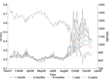
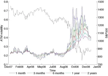
The volatilities of order 2, 3 and 4 are plotted in figures 6(a)-(c). These time series are for the five fixed expirations of 1-3-6 months and 1-2 years. The fixed expiration data was obtained by cubic spline interpolation along the expiration axis. The closing S&P 500 index is plotted for context. The severe market turmoil of September through December stands in stark contrast to the first part of the year. For the sake of expediency we will refer to the last four months of 2008 as “the financial crisis.”

We make a total of eight observations. The first four mirror the points made in Carey (2005) on the basis of snapshot parameter estimates, also for the S&P 500.

Figure 6(a)

Implied base volatility for five fixed expirations S&P 500

[image:11.595.123.497.430.707.2]

Page 11 of 35

Figure 6(b)

Implied skew volatility for five fixed expirations S&P 500

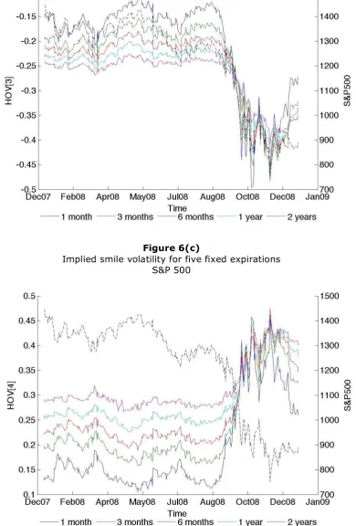
Figure 6(c)

Implied smile volatility for five fixed expirations S&P 500

[image:12.595.109.500.139.716.2] [image:12.595.116.497.443.721.2]

Page 12 of 35

i. Base volatility closely tracks at-the-money volatility. The latter is plotted

in figure 7(a), and is visually indistinguishable from the base volatility time series. To get a clearer picture, consider the ratio of base volatility to at-the-money (ATM) volatility, plotted in figure 7(b). Base volatility is slightly greater for the 1-month expiration, fluctuating around 1.02 times at-the-money volatility; but the situation reverses at about the 3-month mark, whereupon the ratio steadily decreases to about 0.95 at the 2-year mark, with a further dip to below 0.9 during the financial crisis. These conclusions are confirmed by the base and ATM volatility averages, plotted in figure 8.

In addition, the standard deviations of both quantities, also plotted in figure 8, are also broadly similar. The standard deviation of ATM volatility is marginally greater than that of base volatility, a difference that is more pronounced at longer expirations as well as during the financial crisis.

Figure 7(a)

At-the-money Black-Scholes implied volatility for five fixed expirations S&P 500

The dashed line is the S&P 500 index.

ii. Skew and smile volatility have the same order of magnitude and

standard deviation as base volatility. This is revealed by a cursory examination of

[image:13.595.121.496.306.570.2]

Page 13 of 35

Figure 7(b)

Base volatility to at-the-money volatility ratio for five fixed expirations S&P 500

iii. Skew volatility is consistently negative. This is evident from the time series

in figure 6(b). A negative skew volatility implies negative instantaneous skewness. This feature is not surprising, given that negative skewness in the risk-neutral distribution of returns is a well-documented fixture of major equity index markets.

iv. The term structure of skew and smile volatilities is very pronounced.

Considering the first eight months of 2008, this is seen in the time-series in figures 6(b)-(c), as well as in the averages plotted in figure 8. In contrast, the term structure for the base volatilities is essentially flat. Time-inhomogeneity of the parameters is a common feature of option-pricing models featuring a process with independent increments: specifically, the implied skewness and kurtosis increase with expiration. Often this is viewed as evidence that such processes are misspecified, on the grounds that the skewness and kurtosis cannot be expected to increase all the time. However, the presence of parameter bias in a model may or may not be an issue, depending on the specific usage. The Black-Scholes model for instance is still widely used in many markets for trading first-generation derivatives, including the vanilla options considered here.

[image:14.595.117.474.161.423.2]

[image:15.595.102.487.185.494.2]

Page 14 of 35

Figure 8

Mean and standard deviation for at-the-money, base, skew and smile volatilities S&P 500

The bottom figures do not cover the market turmoil of the last four months of 2008, and are thus more representative of normal market conditions.

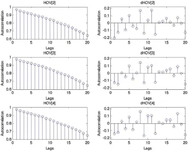
v. Daily changes in the volatilities show mild negative serial correlation.

[image:16.595.105.486.134.440.2]

Page 15 of 35

Figure 9

Correlograms for base, skew and smile volatilities S&P 500

The left column are the ACFs for the volatility time series with fixed expiration 30 days. The right column are the ACFs for the first differences of the same series.

vi. The volatilities are highly cross-correlated. This is true for the absolute

quantities as well as, to a slightly lesser extent, their daily changes. The correlations are plotted in figure 10. For the period prior to the financial crisis, the skew-to-base correlation ranges from 0.96 to 0.98 depending on time to expiration, while the smile-to-base correlation ranges from 0.91 to 0.94. The highest correlation however is between skew and smile volatilities, ranging from 0.97 to 0.99. Cross-correlations for the daily changes follow the same pattern, but with somewhat lower coefficients, and with a marked drop-off at longer expirations: the correlation coefficients are greatest for 3- to 12-month expirations, ranging from 0.93 to 0.98.

[image:17.595.101.484.114.443.2]

Page 16 of 35

Figure 10

Higher-order volatility cross-correlations S&P 500

The left column are the correlations for the base, skew and smile volatilities,

as functions of time to expiration. The right column are the correlations for

daily changes in base, skew and smile volatilities, as functions of time to expiration. The bottom figures do not cover the financial crisis of the last four month of 2008, and are more representative of normal market conditions.

vii. Instantaneous skewness and kurtosis are surprisingly stable. This point

is essentially a corollary to point (vi). Figure 11(a) plots the skew-to-base ratio, which we defined as average instantaneous skewness. This ratio fluctuate within well-defined ranges, which show a strong expiration dependency. Skew volatility ranges in magnitude from 60-70% of base volatility at the 1-month expiration mark, to 105-115% of base volatility at the 2-year mark. The financial crisis appears to result in a slight increase in the standard deviation of the ratio, but overall does not appear to push it in one direction or the other.

Page 17 of 35

Figure 11(a)

Instantaneous skewness for five fixed expirations S&P 500

Figure 11(b)

Instantaneous kurtosis for five fixed expirations S&P 500

[image:18.595.119.500.123.719.2] [image:18.595.122.495.466.732.2]

Page 18 of 35

viii. Changes in the volatilities are correlated with daily returns. It is a stylised fact of equity index markets that changes in at-the-money volatility are negatively correlated with index returns: positive (negative) returns tend to be associated with decreases (increases) in implied volatility. Table 1 reports the correlation coefficients between daily returns and daily changes in base, skew and smile volatilities, for five fixed expirations.

Given the smilarity between ATM volatility and base volatility, it is not surprising that the latter should display a high negative correlation with daily returns, ranging from -0.91 to -0.94. This association is confirmed by figure 12(a), a scatter plot of daily returns3 _{versus daily changes in 1-month base volatility. Based on the best-fit line, an}

index return of +/- 1% is associated with an (absolute) change in base volatility of -/+ 1.23%. The R2 for this regression is 0.83.

Changes in skew and smile volatilities are also correlated with returns. This was expected since, as noted above, daily changes in the volatilities are cross-correlated. The correlation between index returns and changes in skew volatility ranges from +0.83 to +0.90 (table 1), and the best fit line in figure 12(b) suggests an (absolute) change in skew volatility of +/- 0.66% for every +/- 1% index return, with an R2 of 0.73. The correlation between index returns and changes in smile volatility ranges from -0.77 to -0.88 (table 1), and the best fit line in figure 12(c) suggests an (absolute) change in skew volatility of -/+ 0.60% for every +/- 1% index return, with an R2 of 0.69.

Table 1

Correlation between daily returns and daily changes in the volatilities, for five fixed expirations.

S&P 500

Correlation between daily returns and daily changes in …

Time to

expiration Base

volatility

Skew volatility

Smile volatility

1 month -0.9130 0.8553 -0.8333

3 months -0.9325 0.8877 -0.8574

6 months -0.9316 0.8707 -0.8471

1 year -0.9351 0.9028 -0.8849

2 years -0.9141 0.8297 -0.7748

3

Page 19 of 35

Figure 12(a)

Daily changes in base volatility versus daily returns, S&P 500

The best fit line has slope=-1.23, intercept=0.00, and R2=0.83.

Note: the returns used here are synthetic—see footnote 1.

Figure 12(b)

Daily changes in skew volatility versus daily returns, S&P 500

The best fit line has slope=0.66, intercept=0.00, and R2=0.73. Note:

[image:20.595.122.462.110.373.2] [image:20.595.121.461.469.733.2]

Page 20 of 35

Figure 12(c)

Daily changes in smile volatility versus daily returns, S&P 500

The best fit line has slope=-0.60, intercept=0.00, and R2=0.69.

Note: the returns used here are synthetic—see footnote 1.

3. EURUSD 2006 TIME SERIES

The data, obtained from the British Bankers Association (BBA), consists of a set of quotes for each of 253 business days in 2006. Each set comprises an at-the-money, a 25-delta risk-reversal, and a 25-delta strangle volatility, for fixed expirations of 1, 3 and 12 months. These volatility quotes were converted to option prices as detailed in Appendix 3. We used USD and EUR Libor as interest rates. As with the S&P 500 data, the model was calibrated to option prices using squared pricing errors. However, since the number of free parameters in our formula (base, skew and smile volatility) matches the number of inputs (the three volatility quotes), the fit to market prices is exact.

[image:21.595.123.459.153.421.2]

Page 21 of 35

Figure 13(a)

Implied base volatility for three fixed expirations EURUSD

.

Figure 13(b)

Implied skew volatility for three fixed expirations EURUSD

[image:22.595.105.496.109.744.2] [image:22.595.110.496.464.733.2]

Page 22 of 35

Figure 13(c)

Implied smile volatility for three fixed expirations EURUSD

The dashed line is the EURUSD rate.

i. Base volatility closely tracks ATM volatility. As with the S&P 500, base

volatility is visually indistinguishable from ATM volatility, plotted in figure 14(a). The ratio of base volatility to ATM volatility, plotted in figure 14(b), fluctuates between 1.025 and 1.04 for much of 2006, before increasing steeply to the 1.05-1.06 range at the end of the year. The averages for base and at-the-money volatilities, plotted in figure 15, bear this out. As for their standard deviations, they can be observed in figure 15 to be essentially identical.

ii. Skew and smile volatilities have the same order of magnitude and

standard deviation as base volatility. Smile volatility ranges from a low of 3%,

reached at the 1-month expiration, to just under 10%, a high reached at the 1-year expiration, as seen in figure 13(c). This compares to the 6%-10% range achieved by base volatility in figure 13(a). In figure 13(b), skew volatility ranges from -1% to -5% when negative (i.e. most of the time) and from 1% to 2% when positive. Interestingly, when skew volatility changes sign, it does so abruptly and without pausing in the [-1%, +1%] interval.

[image:23.595.117.493.157.423.2]

Page 23 of 35

Figure 14(a)

At-the-money Black-Scholes implied volatility for three fixed expirations EURUSD

The dashed line is the EURUSD rate.

Figure 14(b)

[image:24.595.111.493.124.389.2] [image:24.595.81.430.495.747.2]

Page 24 of 35

iii. Skew volatility alternates between positive and negative. While skew

volatility is negative during most of 2006, indicating negative skewness in EURUSD, two short episodes in which it turns positive can be observed in figure 13(b). These episodes appear to last about a month each, and seem to signal the two major upward moves in EURUSD that occur during the year: the first from 1.20 to 1.28 (March-May), and the second from 1.26 to 1.30 (October-December). It may be that they correspond to the building up of speculative positions in anticipation of the price moves to follow. We observe that Bates (1991) also notes a marked change in skewness prior to the 1987 stockmarket crash.

iv. The term structure of skew and smile volatilities is very pronounced. For

smile volatility, the term structure is very steep, as can be seen both in the time-series in figures 13(b)-(c), and in the averages plotted in figure 15. From a mean value of 4% at the 1-month expiration, it rises to almost 9% at the 1-year mark. In contrast, base volatility has a more modest upward slope, starting at 8% and ending at (coincidentally) 9%.

[image:25.595.102.486.431.739.2]

Skew volatility also has a term structure that increases with time to expiration, albeit to a lesser extent. Because of the intermittent changes of sign, this is not so apparent in figure 15, which plots the mean. In the time-series chart in figure 13(b) however, we see that during periods when EURUSD is range-bound (e.g. May-September), 1-month skew volatility is about 1% less (in magnitude) than that at the 3-month mark, which in turn is 1% less than 1-year skew volatility.

Figure 15

[image:26.595.107.490.182.487.2]

Page 25 of 35

Figure 16

Correlograms for base, skew and smile volatilities EURUSD

The left column are the ACFs for the volatility time series with fixed expiration 1 month. The right column are the ACFs for the first differences of the same series.

v. Daily changes in skew volatility show mild serial correlation, but base

and smile volatilities show none. Figure 16 plots the autocorrelations for the volatility

[image:27.595.103.486.171.483.2]

Page 26 of 35

Figure 17

Higher-order volatility cross-correlations EURUSD

The left column are the correlations for the base, skew and smile volatilities,

as functions of time to expiration. The right column are the correlations for

daily changes in base, skew and smile volatilities, as functions of time to expiration.

vi. Base and smile volatilities are highly correlated, while skew volatility is

largely independent. This holds both for the absolute quantities as well as for the daily

Page 27 of 35

Figure 18(a)

Instantaneous skewness for five fixed expirations EURUSD

Figure 18(b)

Instantaneous kurtosis for five fixed expirations EURUSD

[image:28.595.120.494.124.390.2] [image:28.595.122.494.422.723.2]

Page 28 of 35

vii. Instantaneous skewness is variable and changes sign, while

instantaneous kurtosis is stable. Figure 18(a) plots the skew-to-base ratio. Similarly

to the skew volatility time-series, instantaneous skewness is negative over much of the year, except for a positive episode at the beginning (especially over February) and over the month of October. These positive episodes coincide with troughs in the time-series for EURUSD, subsequent to which there is an abrupt rise in the exchange rate. Over the rest of the year, instantaneous skewness appears to have a term structure that increases with time to expiration. In contrast, instantaneous kurtosis in figure 18(b) is stable over the entire year, albeit with a mild upward drift. The term structure is very pronounced, rising from about 0.5 at the 1-month mark to 1 at the 12-month mark.

viii. Daily changes in the volatilities are largely uncorrelated with daily

returns. Table 2 reports the correlation coefficients between daily returns and daily

changes in base, skew and smile volatilities, for three fixed times to expiration. In contrast to the S&P 500, the correlation coefficients are small and no greater than 0.25 in magnitude. For the sake of symmetry with our treatment of the equity index, we plot daily returns versus daily changes in 1-month base, skew and smile volatility, in figures 19(a)-(c). The weakness of the association is confirmed by an R2 statistic that is close to zero in all three cases.

Table 2

Correlation between daily returns and daily changes in the volatilities, for three fixed expirations.

EURUSD

Correlation between daily returns and daily changes in …

Time to

expiration Base

volatility

Skew volatility

Smile volatility

1 month 0.2484 -0.1986 0.2400

3 months 0.1989 -0.1553 0.1202

Page 29 of 35

Figure 19(a)

Daily changes in base volatility versus daily returns, EURUSD

The best fit line has slope=0.06, intercept=0.00, and R2=0.06. The

volatility series used is for 1-month expirations.

Figure 19(b)

Daily changes in skew volatility versus daily returns, EURUSD

[image:30.595.112.471.109.392.2] [image:30.595.112.466.476.745.2]

Page 30 of 35

Figure 19(c)

Daily changes in smile volatility versus daily returns EURUSD

[image:31.595.112.464.224.509.2]

Page 31 of 35

APPENDIX 1: CHARACTERISTIC FUNCTION OF LOG RETURNS

Here we derive the characteristic function of log returns from Section 1. To avoid repeated technical digressions, we group some auxiliary results below, which can be skipped with no loss of intuition.

There exists a

!

_>

0

_{such that}

!

X

u

X

u

<

1

whenever

!

u

<

"

. (R1)

!

_X

u

X

u

(

)

j+1

<

!

_X

u

X

u

(

)

j

<

₁

and

lim

j!"

#

_X

u

X

u

(

)

j

=

0

_,

!

u

_<

"

_{. (R2)}

!

j+1,u j+1

<

!

j,u j

<

1

and

lim

j!"

#

j,u j

=

0

,

!

u

_<

"

. (R3)

!

j+1,u j+1

<

!

j,u j

<

1

and

lim

j!"

#

_j,uj

₌

0

. (R4)

!

_j ,u j

du

t T

"

<

!

j,u j

du

t

T

"

<

1

,

j

₌

1, 2,...

,

!

u

_<

"

. (R5)

!

_jj_,u

du

t T

"

=

lim

#u$0

%

j,u

j

_#

u

u

&

. (R6)

The series

z

j

!

"#

$

%&

(

'

X

u

X

u

)

j

j=1

n

(

,

n

₌

1, 2,...

converges absolutely,

!

u

_<

"

,

z

_!

C

. (R7)

The series

z

j

!

"#

$

%&

'

j,u,(u

j

₍

u

j=1

n

)

,

n

₌

1, 2,...

converges uniformly in

!

u

_<

min

₍

"

,1

₎

,

z

_!

C

_{. (R8)}

The series

z

j

!

"#

$

%&

'

j,u

j

_du

t

T

(

j=1

n

)

,

n

₌

1, 2,...

converges absolutely,

z

_!

C

_{. (R9)}

(R1) restates an assumption from Section 1. (R2)-(R4) each follow from the preceding result with no difficulty. (R5) holds by the monotonicity property of integrals. (R6) holds since

!

j,u j

_"

u

=

#

j,u j

_"

u

+

o

₍

"

_u

₎

and by (R4). (R7) holds by the ratio test using (R1). (R8) holds by the Weierstrass M-test since:

z

j

!

"#

$

%&

'

j,u

j

₍

u

_<

z

j

!

"#

$

%&

=

M

j

and the partial sums

!

_j

M

_j converge (absolutely) by the ratio test. (R9) holds by the ratio test using (R5).

Moving on to the derivation of the c.f., we assume that

!

u

<

min

(

"

,1

)

. Note first that:

E

_t

!

_"

(

X

_T

X

_t

)

z

#

_$

=

E

_t

(

X

_u+%u

X

_u

)

z

u

&

!

"

'

#

$

(

=

E

_u

!

_"

(

X

_u+%u

X

_u

)

z

#

_$

u

Page 32 of 35

where the product is over the time indices

u

₌

t

,

t

₊

!

u

,...,

t

₊

n

!

u

₌

T

_{. Here we used the law}

of iterated expectations, together with the assumption that the relative increments are market-independent. Now:

X

u+!u

X

u

(

)

z

=

(

₁

+

!

X

u

X

u

)

z

=

₁

+

z

j

"

#$

%

&'

(

!

X

u

X

u

)

j

j=1

(

)

,

where we have used the identity:

1

+

!

(

)

z

=

₁

+

z

j

"

#$

%

&'

!

j

j=1

(

)

,

!

<

1

.

Then by (R7):

E

u

(

X

u+!u

X

u

)

z

=

1

+

E

u

z

j

"

#$

%

&'

(

!

X

u

X

u

)

j

(

)

*

+

,

-j=1

.

/

=

1

+

z

j

"

#$

%

&'

0

j,u,!u

j

_!

u

j=1

.

/

. (A1.2)

Combining (A1.1) and (A1.2) gives:

E

_t

_"

!

(

X

_T

X

_t

)

z

#

_$

=

1

+

z

j

%

&'

(

)*

+

j,u

j

,

u

j=1

-.

!

"

/

#

$

0

u

1

. (A1.3)

Observe next that:

1

+

z

j

!

"#

$

%&

'

j,u

j

₍

u

j=1

)

*

=

exp

o

(

(

u

)

+

z

j

!

"#

$

%&

'

j,u

j

₍

u

j=1 )

*

+

,

-

.

/

0

, (A1.4)

where

o

(

!

u

)

represents terms which vanish with

!

u

faster than

!

u

(that is,

o

₍

!u

₎

!u

"

0

_as

!

u

"

0

). Replacing (A1.4) into (A1.3) and simplifying yields:

E

_t

!

_"

(

X

_T

X

_t

)

z

#

_$

=

exp

o

(

%

u

)

%

u

(

T

&

t

)

+

z

j

'

()

*

+,

-

j,u

j

_%

u

j=1 .

/

u

/

!

"

0

#

$

1

. (A1.5)

By the definition of instantaneous volatility, along with (R3), (R6), (R8) and (R9):

lim

!u"0

z

j

#

$%

&

'(

)

j,u

j

_!

_u

=

z

j

#

$%

&

'(

!

lim

u"0

)

j,u

j

_!

_u

u

*

j=1

+

*

j=1

+

*

u

*

=

z

j

#

$%

&

'(

,

j,u

j

_du

t

T

-j=1

+

*

.

Thus, taking the limit

!

u

"

0

_{in (A1.5) gives:}

E

t

(

X

T

X

t

)

z

!

"

#

$

=

exp

z

j

%

&'

(

)*

+

j,u

j

du

t T

,

j=1

-.

.

Setting

z

₌

i

!

yields the c.f.

! "

( )

=

E

Page 33 of 35

APPENDIX 2: INSTANTANEOUS MOMENTS AND CUMULANTS

The raw moments

µ

j and cumulants

c

j of a random variable satisfy the relation:

µ

_j

=

c

_j

+

j

!

1

k

!

1

"

#$

%

&'

µ

j!k

c

k k=1

j!1

(

(A2.1)

(Stuart and Ord (1994), p.119). Let

m

_j denote the

j

-th infinitesimal moment of a stochastic process; that is, the

j

-th raw moment of the process increment over an interval of time

!t

has the form

µ

j

=

m

j

!

t

+

o

( )

!

t

. To prove that

m

j is also the

j

-th

infinitesimal cumulant we need to show that:

c

n

=

m

n

!

t

+

o

( )

!t

(A2.2)

for every

n

₌

1, 2,...

. We proceed by induction. Note first that equation (A2.2) holds for

n

₌

₁

_{by virtue of the identity}

_µ

1

=

c

1. Next, suppose that (A2.2) holds for

n

=

j

!

1

. Then

(A2.1) reads:

c

_j

=

m

_j

!

t

+

o

( )

!

t

"

j

"

1

k

"

₁

#

$%

&

'(

)*

m

k

!

t

+

o

( )

!

t

+,

)*

m

j"k

!

t

+

o

( )

!

t

+,

k=1

j"1

-

.

Page 34 of 35

APPENDIX 3: FX MARKET QUOTES

The FX option quotes are handled as follows. Let ATM, RR and STR denote respectively the at-the-money, risk-reversal and strangle volatility quotes. The implied volatilities for the 25 delta call and (-)25 delta put are computed as:

!

_C

₌

ATM

₊

STR

₊

1

2

RR

!

_P

₌

ATM

₊

STR

"

1 2

RR

as per the BBA documentation, Wystup (2006) and the treatment in Carr and Wu (200X).4

For EURUSD, the premium currency is USD, and the deltas are of the regular spot kind. To determine the strike prices corresponding to a given delta level, we use the following formula:

K

=

F

exp

!"# $

N

!1

"

e

rf$

%

(

)

+

1

2

#

2

_$

&

'

(

)

,

where

!

₌

₁

for a call option,

_!

₁

for a put. For example, the ATM strike is

K

=

F

exp

1

2

!

2

_"

#$

%&

, corresponding to the ATM

!

₌

1 2

"

e

rf#_{. For more details see Reiswich and}

Wystup (2009).

4

Page 35 of 35

REFERENCES

Abramovitz, M. and I. Stegun (1972) Handbook of Mathematical Functions, 10th printing, National Bureau of Standards, United States Department of Commerce.

Babbs, S. and M. Selby (1998) Pricing by arbitrage under arbitrary information,

Mathematical Finance 8(2), 163-168.

Bates, D. (1991) The crash of ’87: Was it expected? Evidence from options markets,

Journal of Finance46(3), 1009-1044.

Black, F. and M. Scholes (1973) The pricing of options and corporate liabilities, Journal of

Political Economy81(3), 637-654.

Brody, D., L. Hughston and A. Macrina (2007) Information-based asset pricing,

International Journal of Theoretical and Applied Finance 11(1), 107-142.

Carey, A. (2005) Higher-order volatility, working paper, SSRN e-library.

Carey, A. (2006) Higher-order volatility: dynamics and sensitivities, working paper, SSRN e-library.

Carr, P. and L. Wu (2007) Stochastic skew in currency options, Journal of Financial

Economics 86, 213-247.

Daglish, T., J. Hull and W. Suo (2007) Volatility surfaces: theory, rules of thumb, and empirical evidence, Quantitative Finance 7(5), 507-524.

Gikhman, I. and A. Skorokhod (1972) Stochastic Differential Equations, Springer-Verlag.

Hakala, J., R. Stuart and T. Hamosfakidis (2008) FX derivatives, presentation slides, Standard Chartered Bank.

http://www.mathfinance.com/workshop/2008/papers/hakala/slides.pdf

Johannes, M. (2004) The statistical and economic role of jumps in continuous-time interest rate models, Journal of Finance59(1), 227-260.

Merton, R. (1973) Theory of rational option pricing, Bell Journal of Economics and

Management Science 4(1), 141-183.

Merton, R. (1976) Option pricing when underlying stock returns are discontinuous,

Journal of Financial Economics 3(1-2), 125-144.

Reiswich, D. and U. Wystup (2009) FX volatility smile construction, working paper, Frankfurt School of Finance and Management.

Stuart, A. and K. Ord (1994) Kendall’s Advanced Theory of Statistics (Volume 1), 6th edition, Arnold.