http://dx.doi.org/10.4236/ojs.2016.63041
How to cite this paper: Marano, G., Boracchi, P. and Biganzoli, E.M. (2016) Estimation of the Piecewise Exponential Model by Bayesian P-Splines via Gibbs Sampling: Robustness and Reliability of Posterior Estimates. Open Journal of Statistics, 6,
Estimation of the Piecewise Exponential
Model by Bayesian P-Splines via Gibbs
Sampling: Robustness and Reliability of
Posterior Estimates
Giuseppe Marano1, Patrizia Boracchi2, Elia M. Biganzoli1,2*
1Unit of Medical Statistics, Biometry and Bioinformatics, Fondazione IRCCS Istituto Nazionale dei Tumori di
Milano, Milan, Italy
2Laboratory of Medical Statistics, Biometry and Epidemiology “G. A. Maccacaro”, Department of Clinical
Sciences and Community Health, University of Milan, Milan, Italy
Received 1 April 2016; accepted 19 June 2016; published 22 June 2016
Copyright © 2016 by authors and Scientific Research Publishing Inc.
This work is licensed under the Creative Commons Attribution International License (CC BY).
http://creativecommons.org/licenses/by/4.0/
Abstract
In the investigation of disease dynamics, the effect of covariates on the hazard function is a major topic. Some recent smoothed estimation methods have been proposed, both frequentist and Baye-sian, based on the relationship between penalized splines and mixed models theory. These ap-proaches are also motivated by the possibility of using automatic procedures for determining the optimal amount of smoothing. However, estimation algorithms involve an analytically intractable hazard function, and thus require ad-hoc software routines. We propose a more user-friendly al-ternative, consisting in regularized estimation of piecewise exponential models by Bayesian P-splines. A further facilitation is that widespread Bayesian software, such as WinBUGS, can be used. The aim is assessing the robustness of this approach with respect to different prior functions and penalties. A large dataset from breast cancer patients, where results from validated clinical studies are available, is used as a benchmark to evaluate the reliability of the estimates. A second dataset from a small case series of sarcoma patients is used for evaluating the performances of the PE model as a tool for exploratory analysis. Concerning breast cancer data, the estimates are ro-bust with respect to priors and penalties, and consistent with clinical knowledge. Concerning soft tissue sarcoma data, the estimates of the hazard function are sensitive with respect to the prior for the smoothing parameter, whereas the estimates of regression coefficients are robust. In conclu-sion, Gibbs sampling results an efficient computational strategy. The issue of the sensitivity with respect to the priors concerns only the estimates of the hazard function, and seems more likely to
occur when non-large case series are investigated, calling for tailored solutions.
Keywords
Survival Analysis, Hazard Smoothing, Bayesian P-Splines, Piecewise Exponential Model, Time-Dependent Effects
1. Introduction
In several bio-statistical applications on censored follow-up time data, the interest lies mainly on the prognostic role of clinical/biological covariates. To such end, non-parametric and semi-parametric methods have been pre-ferred over parametric ones. The most widely adopted tool is the Cox model, which avoids any assumption of the functional form of the hazard function on time. However, such feature is not useful if the interest lies on in-vestigating the shape of the hazard or in predictive modeling. A solution was to include a flexible expression of the hazard function directly in the likelihood function for survival models (e.g. [1]-[3]): this was considered since 1995 by Herndon and Harrell, who used restricted cubic splines ([4]).
Spline functions require the definition of the number of basis and position of spline knots. This can be diffi-cult when the phenomenon under investigation presents complex features, such as a non-monotonic shape of the hazard with multiple peaks, or time dependent covariate effects. Penalized splines (P-splines) may be of advan-tage, since they avoid an arbitrary definition of spline bases, by using a high number of bases and eventually knots placed on a grid of equally spaced points. Furthermore, the degree of smoothing is controlled by regula-rized estimation, thus reducing the effective number of model degrees of freedom, and, therefore, giving a sys-tematic method for the bias variance trade-off. Different kinds of penalization can be applied, potentially giving different results. The most common method has been proposed by Eilers and Marx ([5]), based on B-splines re-gularized with finite difference penalty functions (also called “roughness penalties”).
Penalized methods for estimating survival models have been described in the frequentist framework by Kauermann ([6]), amongst others. The proposal is based on specifying the hazard function through flexible po-lynomials, including directly such function in the likelihood function for survival data, and treating the coeffi-cients of the polynomials as random effects. This approach allows resorting to the relationship between P-splines and mixed model theory (cfr: [7]). However, the implementation of the above method can be cumber-some, because it requires the maximization of a likelihood function that includes a complex integral without a closed-form solution.
For what concerns penalized estimation methods in general, the confidence intervals based on the multivariate normal distribution of the estimates have unsatisfactory performances, because of penalty-induced biases (cfr: [8]). Imposing a determined penalty is equivalent to specify some prior belief about the characteristics of the best model. In fact, the penalty makes explicit the fact that smooth models are believed to be more likely than “wiggly” ones. This has been a motivating rationale to use Bayesian methods ([9][10]).
Bayesian P-splines have been introduced by Lang and Brezger ([11]). Fahrmeir and Hennerfiend ([12]) dis-cuss their implementation in survival analysis. Dedicated routines are available, for example, in the software package BayesX ([13]). In such a context, point and interval estimates of model parameters and survival func-tions may be obtained in a straightforward way from posterior density samples. To this aim, Markov Chain Monte Carlo (MCMC) methods are needed, but they require efficient sampling algorithms in order to guarantee convergence of the Markov chains, and may be computationally intensive. The estimation method in [12] also deals with the survival likelihood, and, thus, shares the problem of the intractability of the cumulated hazard with the previously cited frequentist methods. In order to solve this problem, specific sampling schemes have been adopted for computation. Therefore, a dedicated software must be used to fit models in practice.
be-cause of their link with the Poisson distribution (GLM family of distributions). The PE family of models has been a basic block in past works ([14][15]) for developing useful strategies of model building and assessment in the competing risks setting. Recognizing the advantage of penalized splines, recently ([16]) we described in de-tail the specification of a Bayesian PE model with a hazard function modeled by penalized splines for the analysis of univariate survival times. The model is analogous to the general model in [12], but it is provided of a tractable likelihood function. In contrast with earlier approaches, the model can be fitted through general rou-tines for estimating GLM hierarchical models: therefore, general Bayesian software can be used for computa-tion.
In [16], we described the implementation of Bayesian P-splines method for obtaining estimates of the hazard, of regression coefficients and survival probabilities. Examples have been given of estimation of models with a second order difference penalty and two distinct priors for the smoothing parameter. In this work we considered an extended expression of the model above, allowing regularized estimation of non-linear and time-varying ef-fects of prognostic factors. Furthermore, we extended the evaluation of the robustness of the Gibbs sampling es-timation method. To such end, we fitted several competing models, with different combinations of penalties and a more extensive set of prior densities, to two datasets, from breast cancer and soft tissue sarcoma patients, re-spectively. The adequacy of the competing models was assessed through the deviance information criterion (DIC) ([17]) using the standard expression for Poisson regression models. Furthermore, the reliability of the method was preliminarily evaluated by comparing the estimates of the hazard function on a large case series (breast cancer dataset) against benchmark clinical situations derived from literature: i.e. papers on tumor dor-mancy in breast cancer (cfr: [18][19]).
The remainder of this paper is organized as follows. In the method section we illustrate the construction of a general PE model with smooth components for the baseline hazard function, non-linear and/or time-varying ef-fects of covariates. The smooth components above were specified following Eilers and Marx’s approach ([5]). In the subsequent section, results are presented concerning the evaluation of the robustness and the reliability of the estimates. Finally, conclusions and open issues are discussed.
2. Methods
In this section, a brief illustration of the characteristics of the standard PE model, with particular attention to the link with Poisson regression models, is firstly provided. Subsequently, methods for penalized estimation are re-viewed. After this, the Bayesian P-splines estimation method is illustrated, and the general expression of the Bayesian PE models is illustrated. The section ends with two sub-sections concerning, respectively, the practical implementation of Bayesian P-splines and the definition of the DIC.
2.1. Simple PE Model
For univariate, possibly right-censored, survival data, let (Ui, Ci) be the random variables indicating,
respective-ly, failure time and censoring time of the i-th subject. The observed data is represented by: ti = min(ui, ci) and by
the status: vi:vi= 0 if ti = ci and 1 if ti = ui. Let Xi (p × 1 vector) indicate the set of covariates of subject i recorded
at the beginning of the study. In the standard PE model the follow-up time is partitioned into a fixed set of H in-tervals: {Th = [τh−1, τh); τ0 = 0, h=1,,H} and it is assumed that the time to failure U has an exponential
dis-tribution within each interval, whose parameters depend on the time intervals and the covariates. In the simplest case of proportional hazards, the relationship between the hazard function of the PE model and the covariates:
(
|)
PE t Xi
λ ; is expressed as follows:
(
)
(
(
)
)
(
T)
1
| exp , 1, , ;
H
PE i h h i
h
t X I t T X i n
λ λ β
=
=
∑
∈ = (1)where: λ1,,λH are the unknown parameters of the baseline hazard function; β is the p × 1 vector of
re-gression coefficients; and I(t∈Th) is an indicator function being equal to 1 if τh−1 ≤ t < τh and 0 otherwise.
For right censored data the likelihood function has the general form:
(
)
(
(
)
)
(
(
)
)
1
, | , , | iexp | ;
n
v
i i i i
i
L λ β t v X λ t X t X
=
=
∏
−Λ (2)the covariates. The function
(
)
(
)
0
| i t | i d
t X λ s X s
Λ =
∫
is the cumulative hazard. This likelihood resembles the likelihood of a Poisson random variable Vi, with mean parameter µi= Λ(
ti|Xi)
. By substituting λ(
ti|Xi)
inexpression (2) with λPE
(
ti|Xi)
(expression (1)), the likelihood becomes:(
)
(
(
)
)
(
(
)
)
1 1
, ; , , exp exp exp ;
i ih
H
n v
T T
PE h i h i ih
i h
L λ β V X λ X β λ X β
= =
∆ =
∏∏
− ∆ (3)where for each subject i there is a product of Hi terms, Hi being the number of intervals in which the subject is
followed. In the expression above, vih is the status of the i-th subject within the interval Th (0 = alive or censored,
1 = failed); Δih is the time spent in Th by the subject.
From expression (3) it may be seen that LPE is proportional to the product of Poisson likelihoods for Vih with
mean parameters: µih=λhexp
(
XiTβ)
∆ih. As a consequence, the expression of the Poisson regression model is:( )
( )
T( )
; log log , 1, , , 1, , ;
ih ih ih h i ih i
V ∼POISSON µ µ =α +X β+ ∆ i= n h= H (4)
where αh = log(λh) are log-hazard parameters, and the term log(Δih) is an offset.
For fitting the PE model through model (4) as Poisson regression model, an augmented dataset must be de-rived from the original one. To such end, the data of each subject needs to be replicated for each interval in which it is followed. For each replicate, a row data indicating subject covariates, time interval and the status of the subject within the interval must be created for h=1,,Hi. Also, H dummy variables must be included for
estimating the parameters αh. Time varying effects of, say, a variable Z1, may be easily included through a
prod-uct of the dummy variables above and Z1. For more details about the PE model we refer to Rodríguez-Girondo et al. ([20]) and to the textbooks of Lawless ([21]) and Congdon ([22]) for more methodologically oriented dis-cussions.
2.2. Hazard Smoothing
To obtain an interpretable shape of the hazard, a method for smoothing the time terms of the piecewise linear predictors is needed. Spline functions are the widest applied approaches. A spline function is a flexible poly-nomial constructed by joining ordinary polypoly-nomials within a set of intervals. For the time to event T, let’s con-sider a generic partition of the range of possible values formed by a set of K adjacent intervals, say:
( )
; 1, ,j j
I =I T j= K; the extremes of the intervals are called knots. A spline of degree p may then be written as:
( )
; j( )
; for j, 1, ,spf t p =P t p t∈I j= K
where Pj(t;p) are polynomials of the same degree p. Usually, specific constraints are used for guaranteeing the
continuity of spf(t;p) in the knots, so that to impose a smooth shape to the function.
Several classes of splines have been proposed in literature. Basis splines (B-splines) are the most widely used by statisticians, because of their favorable properties ([23]). The general expression of a B-spline is:
( )
T( )
1
; ; ;
M
m m
m
Bspf t p B γ B t p γ
=
= =
∑
(5)where: B=
(
B t p1( )
; ,,BM( )
t p;)
T is a M × 1 vector of spline bases, and(
)
T 1, , Mγ = γ γ is the vector of associated coefficients (M × 1). The expressions of the bases Bj(t; p) for differing values of p are derived by a
recursive formula that is not of interest here. Usually, cubic splines are considered.
To such end, penalized splines (P-splines) have been proposed in the GLM regression context by Eilers and Marx ([5]). The method is based on penalized estimation of the coefficients of B-spline functions using finite difference penalties (or roughness penalties). It may be applied in a natural fashion for regularizing the estimates of the hazard function. In the PE model, the baseline hazard function is piecewise constant. Such a function is a particular case of B-splines, given for p = 0. Thus we can write for each h: αh =BT0α, and substituting this term in expression (4). Thus for applying Eilers and Marx’s method, a penalization term on the coefficients
1, , H
α α is needed. By referring to the GLM model (4), the estimates are determined by maximizing the pe-nalized log-likelihood l′
(
α β, ; , ,V ∆ X)
:( )
(
)
(
)
(
) (
)
, 2 T , ˆˆ, arg max , ; , ,
arg max , ; , ,
2
POISSON d d
l V X
l V X D D
α β
α β
α β α β
ϕ
α β α α
′
= ∆
= ∆ − (6)
where lPOISSON
(
α β, ; , ,V ∆ X)
is the log-likelihood for model (4), φ2 is a smoothing parameter, and Dd repre-sents the finite differences operator of order d: T
{
( )
}
1, , dd h
h d H
D α α
= +
= ∆
. More specifically, Δ
d
is defined as
the functional that maps any variable into its finite differences: for d = 1: ∆1
( )
αh =αh−αh−1; h=2,,H; for d = 2: ∆2( )
αh = ∆ ∆1(
1( )
αη)
=αh−2αh−1+αh−2; h=3,,H; for a generic value of d:( )
1(
1( )
)
d d
h h
α − α
∆ = ∆ ∆ ; h= +d 1,,H Therefore, since stronger irregularities of the hazard correspond to
higher finite differences of the parameters αh, the “effect” of the penalty term:
(
) (
)
2 T
2 Dd Dd
ϕ α α
− ; on the pe-
nalized log-likelihood function consists in supporting models with more regular hazard shapes over models with more irregular ones (expression (6)). The smoothing parameter φ2 is an additional parameter required for “tuning” the trade-off between model fit and model smoothness.
2.3. Bayesian P-Splines
The Bayesian P-splines method ([11]) is based on a hierarchical model for expression (4) with non informative priors for the regression coefficients
( )
β and a Gaussian Random Walk (RW) prior of order d for the coeffi-cients of the hazard function (B-spline), conditional to a smoothing parameter τ2. The general expression of the RW prior is the following:T 2
2
1
| exp ;
2 Pd
α τ α α
τ
∝ −
(7) where: Pd =D DdT d. By assuming τ
2
= 1/φ2, the argument of the exp() function above closely resembles the pe-nalty term in expression (6).
By indicating the RW prior with the term: RW(τ2, Pd), a general expression of the PE model with a regularized
hazard function is:
( )
( )
( )
(
)
2T T
0
2 2 2
; log log
| , ;
ih ih ih i ih
d
V POISSON B X
RW P
β
τ
µ µ α β
β π
α τ τ τ π
∼ = + + ∆ ∼ ∼ ∼ (8)
where: B0 is the vector form of a B-spline of degree 0 defined on the intervals: T1,,TH of the follow-up
pe-riod, and πβ and πτ2 are generic prior densities for the regression coefficients and the smoothing parameter. Further details on these priors will be given in a following subsection. For the former prior, univariate diffuse Gaussian densities are typically used in literature. For πτ2, the most common choice is an inverse-gamma den-sity with a high variance. However, in principle every prior for variance parameters in hierarchical models could be used ([26]). Furthermore, it has been pointed out (e.g.: [27]) that the choice of πτ2 may have an unwanted influence on the posterior estimates: thus a sensitivity analysis is recommended in effective applications.
The expression above defines a hierarchical (mixed effect) Poisson model where the log-hazard parameters:
1, , H
sampling algorithms for hierarchical GLM models. In particular, software based on Gibbs sampling (e.g. Win-BUGS) are an adequate choice, which facilitates the application of a global strategy for building useful models. We provided elsewhere the code for the estimation of model (8) through WinBUGS; other examples have been given as accompanying material for the paper by Murray et al. ([28]).
2.4. General PE Model with Smoothed Components
Expression (8) may be easily extended for penalized estimation of possible non-linear and/or time-dependent effects of covariates, by including in the model expression, for each covariate, a basis spline function (B-spline polynomial) and an additional RW prior for each covariate. From now on, we will indicate with: Z11,,Z1p
the covariates with time-dependent effects; by Z21,,Z2q the covariates with non-linear effects, and with X the matrix including the values of covariates with unpenalized effects. The general expression of the PE model with regularized effects is the following:
( )
( )
( )
( )
(
)
( )(
)
( )(
)
2 2 2 TT T T
0 1 , 0 1 2 , 2
1 1
2 2 2
2 2 2
1
2 2 2
2
log log
| , ;
| , ; ; 1, ,
| , ; ; 1, ,
j
p j
ih ih
p q
ih j i j j i j i ih
j l
d
j
j j d j
j
p l
p l p l d p l
l
V POISSON
B z B B z X
RW P
RW P j p
RW P l q
β
τ τ
τ
µ
µ α γ γ β
β π
α τ τ τ π
γ τ τ τ π
γ τ τ τ π
+ = = + + + + ∼ = + + + + ∆ ∼ ∼ ∼ ∼ ∼ = ∼ ∼ =
∑
∑
(9)The time-dependent effects for each covariate are: z1 ,j iBT0γ1j; j=1,,p. Thus, for each Z1j, its values
multiplied for a piecewise constant function: B0Tγ1j; in the parameters
(
)
T 1j 1 ,1j , , 1 ,j Hγ = γ γ . This enables the effect of each Z1j to vary in each interval Th of the original partition of the follow-up:
T T
0 1 ,j i 0 1j h 1 ,j i 1 ,j h
B α+z B γ =α +z γ for t∈Th. On the other hand, the effects of Z21,,Z2q have been represented trough the general expression of B-splines (expression (5)), with the vector B z
( )
2 ,l i T including the spline basis of Z2l calculated for the i-th individual. Thus, in this case the degree and the knots of each spline are fixedfol-lowing conventional rules (cfr: [5]).
2.5. Implementation Details
A more detailed discussion is needed concerning the implementation of RW priors in software. From expression (7) it may be seen that RW priors are essentially multivariate Gaussian priors with mean vector 0 and covariance matrix τ2
( )
Pd 1−
Σ = . However, the matrix Pd is rank-deficient. To justify this statement, we recall that
T
d d d
P =D D , where Dd is the finite difference matrix of order d. The rank of Pd equals the rank of Dd (since
rank(MTM) = rank(M) ; M being a generic n × k matrix), and Dd is generally not full-rank, due to the properties
of the finite difference operators.
For the reasons above, the standard densities available in software does not apply to the RW prior. In alterna-tive one can use the CAR function, which is specifically designed for Gaussian autoregressive stochastic processes, and is available in WinBUGS (cfr: [29]). Another alternative that does not require specific software consists in a reparameterization of the hazard parameters α1,,αH in two independent vectors with full-rank
covariance matrices and regular prior densities (see: [30] for details). The reparameterization is based on the following expression:
1 1 2 2
α= Ψα + Ψα ;
where α1, α2 are vectors of length d and H-d, and Ψ1, Ψ2 are matrices of dimensions H × d and H×
(
H−d)
, respectively. Thus, the dimensions of the terms above depends on the choice of the degree d of the penalty func-tion. In particular,
(
T)
1 2 Dd D Dd d−
Ψ = , whereas the expression of Ψ1 is obtained as follows, by matrix algebra argumentations. A useful expression for deriving Ψ1 is:
T 1 0
d
of Ψ1 and Ψ2). This implies that the columns of Ψ1 form a basis for the null space of the finite difference operator Δd (section: hazard smoothing). In practice: for d = 1, the expression becomes:
T
1 0
Dψ = ; ψ =
(
ψ2,,ψH)
T.This implies: Δ1(Ψ
h) = 0; which is satisfied by: ψ1=
(
1,,1)
. For d = 2, the condition: Δ2(ψ ) = 0 is satisfied by ψ1 and by another vector that includes a linear succession: ψ2 =(
1, 2,,H)
. For higher values of d, the columns of Ψ1 will be obtained by including additional vectors, ψ2,,ψd that will include successions of higher order.From the definitions above it follows that the parameters in α1 have a flat prior density, whereas indepen-dent conditional Gaussian priors (conditional to τ2) must be assumed for the parameters in α2. For example, the following expression shows an equivalent reformulation of model (8) that can be readily implemented in Win-BUGS as like as in any other dedicated software:
( )
( )
( )
( )
2T T T
0 1 1 0 2 2
1
2 2
2 2
; log log
; 1, ,
| 0, ; 1, ,
ih ih ih i ih
k
k
V POISSON B B X
const k d
N k H d
β
τ
µ µ α α β
β π α
α τ τ
τ π
∼ = Ψ + Ψ + + ∆
∼
∝ =
∼ = −
∼
(10)
For more general models (expression (9)) the equivalent expressions are obtained straightforwardly.
2.6. Deviance Information Criterion
The DIC is a frequently used tool for comparing the adequacy of competing models (cfr: [17]). For GLM mod-els, it can be considered as a generalization of the Akaike Information Criterion (AIC), and thus it yields a rank-ing of competrank-ing models based on their predictive ability. The general expression is:
( )
2 D;DIC=D θ + p
where: D
( )
θ is the model deviance calculated in the posterior mean of the parameters: θ , pD = −D D( )
θ isa “measure” of the effective degrees of freedom. The DIC is a useful statistic for hierarchical models and, also, for penalized models, for which the traditional measures of model complexity does not apply. Furthermore, the DIC is calculated very easily from the output of Gibbs sampling software. For such reasons, we considered the DIC as an appealing tool for model comparison in this work.
3. Results
3.1. General Plan of Analysis
The Bayesian P-splines method was applied to two datasets on breast cancer and soft tissue sarcoma patients (cfr: [31][32]). The covariates included in the models were fixed a priori and corresponded to well-known prognostic factors for the investigated outcomes. The partition of the follow-up time was based on routine clinical fol-low-up schedules. Moreover, previous experience on breast cancer patients analysis suggested us that narrower intervals do not improve the knowledge of disease dynamics. In the remainder application, there is a higher un-certainty about this issue; however the assumption of a constant hazard between consecutive patient visits is reasonable on clinical grounds.
For the breast cancer dataset only discrete covariates were included: age at diagnosis (≤35 years, 36 - 45 years, 46 - 55 years, 56 - 65 years, >65 years), tumor size (≤0.5 cm, 0.6 - 1.0 cm, 1.1 - 1.5 cm, 1.6 - 2.0 cm, >2.0 cm), nodal status (N−, 1 N+, 2 - 3 N+, ≥4 N+), histologic type (infiltrating intraductal component or infiltrating lobu-lar component: IDC + ILC; extensive intraductal component: EIC; other histology) and tumor site (external, in-ternal or central); according to the original study ([31]). The hazard function was expressed through basis func-tions (expression (10)). We considered both a model without time-varying covariate effects (that is, proportional hazards (PH) model), and a model with a time-varying effect of tumor size.
for the hazard and the regression coefficients have been compared by descriptive methods (tabulation, graphical representation). A more formal comparison was performed using the DIC.
The priors used for defining the competing models were: four inverse-gamma priors for the smoothing coeffi-cients (τ2): Γ−1(a,a) with a = 1, 10−2, 10−4, 10−6; and a uniform prior: U(0,100) for τ. The penalties were specified through finite difference penalties of order 2 and 3. Furthermore, the reliability of the estimation method has been assessed, by comparing the behavior of the estimated hazards against benchmark clinical situations derived from literature ([18][19]).
In the second application (soft tissue sarcoma), the covariates were: age (years) and tumor size (cm) (conti-nuous variables), histologic subtype, grading and surgical margins (microscopic, macroscopic) (categorical va-riables). The classes of categorical covariates corresponded to those used in the original study ([32]). Concern-ing the shape of the hazard, there is no widely accepted knowledge: thus a PE model with a smoothed hazard function (without time-varying covariate effects) was used as a tool for exploratory analysis. The robustness of the estimation method has been assessed following the same strategy illustrated above.
In each application, MCMC sampling was performed by executing WinBUGS under R ([33]), via the R2WinBUGS package ([34]). Subsequent calculations were done in R with the coda package ([35]) added. Posterior estimates were obtained from single chains of length 20,000, with burn-in of 2000 and thinning by 5. Thus, the effective size of the posterior sample was 3600. In each case, standard diagnostic techniques showed appreciable mixing properties of the Markov Chains, and autocorrelations rapidly approaching zero.
3.2. Application 1: Breast Cancer Dataset
3.2.1. PE Model with a Smoothed Hazard Function
The sample included 2010 patients out of 2233 who underwent conservative surgery at Milan Cancer Institute between 1970 and 1987. The outcome considered here was event-free survival (which included: local recur-rences, distant metastases, other primary tumor, death).
Due to the large sample size, a procedure for avoiding an excessive computational burden was required: recall that for fitting the PE model the original dataset must be augmented (methods section). We resorted to a “bin-ning” approach (as, for example, in [36]): the patients were grouped in K groups, identified by the K possible combinations of covariate values observed in the sample (bins). Then, a new dataset of K rows was constructed, including: the total number of subjects in the group; the number of observed events and the total follow-up times for the subjects above; and the set of covariate values corresponding to each bin. The PE models described in the following were then fitted to the binned datasets. The benefits of this procedure increase as the difference n (sample size) and K becomes higher.
For specifying the PE model with a smooth hazard function, the follow-up period was divided in 18 consecu-tive intervals of one year length. The covariates were all categorical. They were included in the expression of the model through dummy variables using the “reference category” coding. By indicating the dummy variables with the letter D, the linear predictor of the model: η = log(μ) was:
( ] ( ] ( ]
( ] ( ] ( ]
T T
0 1 1 0 2 2 AGE 35,45 1 AGE 45,55 2 AGE 55,65 3 AGE 65 4
5 6 7 TSIZE 2.0 8
TSIZE 0.5,1.0 TSIZE 1.0,1.5 1.5,2.0
NODSTATUS 1N 9 NODSTATUS 2-3N 10 NODSTATUS 4 N 11
HIST EIC 12 HI
TSIZE
B B D D D D
D D D D
D D D
D D
η α α β β β β
β β β β
β β β
β
>
∈ ∈ ∈
>
= + = + = +
=
= Ψ + Ψ + + + +
+ + + +
+ + +
+ + ST OTHER= β13+DTSITE INTERNAL OR CENTRAL= β14
(11)
where: AGE, TSIZE, NSTATUS, HIST and TSITE indicate, respectively: age at diagnosis, tumor size, nodal status, histologic type, and tumor site. The intercept corresponds to the first element of the vector α1 (because the first column of Ψ1 is always a constant vector of ones). The model includes 33 parameters: 32 in the linear predictor (18 hazard parameters for the baseline hazard function and 14 for the regression coefficients) plus 1 smoothing parameter.
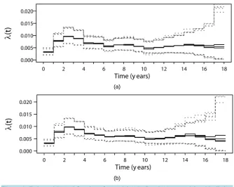
(a)
(b)
Figure 1. Estimated hazard functions for model (11). Panel (a): 5 models with distinct priors for the smoothing parameter and second order difference penalty; Panel (b): 5 models with the same priors and a third order difference penalty. Black solid lines: posterior means; dotted lines: 95% credibility intervals. Covariate values were: Age: ≤35 years, tumor size:
0.5 cm, nodal status: 4 N+, quadrant: external, histology: IDC + ILC.
fixed set of covariate values: age ≤ 35 years, tumor size ≤ 0.5 cm, nodal status = 4 N+, quadrant = external, his-tology = IDC + ILC). As it may be seen, the estimates were practically undistinguishable.
Concerning the clinical interpretation of the function, the shape resulting from Figure 1 showed a major peak within the third year of follow-up, followed by a non constant trend, in which two other peaks could be noticed. This behaviour is consistent with accepted clinical knowledge on breast cancer case series (e.g.: [18][19]), al-though the accuracy of estimates was rather low (especially in the later follow-up period).
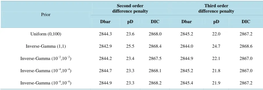
A more formal evaluation of the ten competing models was performed through the DIC. From the values re-ported in Table 1, no relevant differences emerged in terms of model fit (deviance), effective degrees of free-dom (pD) and therefore in terms of overall adequacy (DIC). Thus, in the present example the choice of different
priors and/or penalties had a negligible influence on posterior sample estimates.
3.2.2. PE Model with a Time-Varying Effect of Tumor Size
The specification of the time-varying effect required to include extra basis functions (B-splines of degree 0) for the modalities of tumor size (expression 9). The expression of the linear predictor was specified as discussed in the following. In expression (9) the term: BT0α represents a piecewise constant hazard for patients with tumor size lower or equal 0.5 cm (the reference category), whereas smooth terms of the form: DTSIZE,kBT0γk would
represent (smooth) differences between the hazard of the remainder categories of tumor size (k = 1 - 4) and the previously indicated hazard. We considered more appealing to obtain smooth estimates directly for each hazard function: therefore, we slightly modified the expression:
( ] ( ] ( ]
T T T T T
0 TSIZE 0.5,1.0 0 1 TSIZE 1.0,1.5 0 2 TSIZE 1.5,2.0 0 3 TSIZE 2.0 0 4
B α+D ∈ B γ +D ∈ B γ +D ∈ B γ +D > B γ
into the following one:
( ] ( ] ( ]
T T T T T
0 0 0 0 0
TSIZE 0.5 TSIZE 0.5,1.0 1 TSIZE 1.0,1.5 2 TSIZE 1.5,2.0 3 TSIZE 2.0 4
D < B α+D ∈ B γ +D ∈ B γ +D ∈ B γ +D > B γ .
[image:9.595.145.480.81.347.2]Table 1. Adequacy of the competing models for estimating model (11) Dbar = deviance; pD = effective degrees of freedom;
DIC = Deviance Information Criterion.
Prior
Second order difference penalty
Third order difference penalty
Dbar pD DIC Dbar pD DIC
Uniform (0,100) 2844.3 23.6 2868.0 2845.2 22.0 2867.2
Inverse-Gamma (1,1) 2842.9 25.5 2868.4 2844.0 24.7 2868.6
Inverse-Gamma (10−2,10−2) 2844.2 23.4 2867.5 2844.9 22.1 2867.0
Inverse-Gamma (10−4,10−4) 2844.7 23.3 2868.1 2845.2 21.8 2867.0
Inverse-Gamma (10−6,10−6) 2844.9 23.3 2868.2 2845.4 21.9 2867.2
for tumor size and cell means coding for follow-up time, into a model with cell means coding for both the “fac-tors” above. The final expression of the linear predictor was made similar to expression (10):
( ] ( ] ( ]
1 2
TSIZE 0.5 01 TSIZE 0.5 02 TSIZE 2.0 41 41 TSIZE 2.0 42 42
1 2 3 AGE 65 4
AGE 35,45 AGE 45,55 AGE 55,65
NODSTATUS 1N 5 NODSTATUS 2-3N 6 NODSTATUS 4N 7
HIST EIC 8 HIST OTHER 9 T
D D D D
D D D D
D D D
D D D
η α α γ γ
β β β β
β β β
β β
< < > >
>
∈ ∈ ∈
= + = + = +
= =
= Ψ + Ψ + + Ψ + Ψ
+ + + +
+ + +
+ + +
SITE INTERNAL OR CENTRAL= β10
(12)
Due to the very low frequency of events observed at later times, the follow up was truncated to 15 years (in-stead of 18) for overcoming hard convergence problems of the Markov Chains. After this, a regular behaviour of the chains was shown in each case. Model (12) included a total of 90 parameters, divided in: 75 parameters for the time-varying effect of tumor size; 10 for other regression coefficients and 5 smoothing parameters.
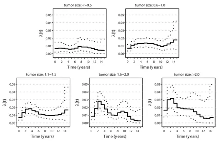
As in the previous section, the estimates of all model parameters were robust with respect to priors and penal-ties. For sake of simplicity, results were reported for only one competing model (uniform prior for the smooth-ing parameters, second order difference penalty). The most evident time-varysmooth-ing effects of tumor size were shown comparing the hazard shapes for tumors sized ≤1.0 cm with the shapes for tumor size: from 1.1 - 1.5 cm to >2.0 cm (Figure 2). A high peak after the second year of follow-up emerged clearly only for tumor size ≥1.1.
cm; a second evident peak may be seen at the 10th year of follow-up, for tumor size between 1.6 cm. and 2.0 cm. These characteristics are, again, consistent with the clinical experience. Even though the estimates for tumor size >2.0 cm were inaccurate. This outcome was likely due to a low number of events occurred in the later fol-low-up.
3.3. Application 2: Soft Tissue Sarcoma Data
Data were collected from a case series of 192 subjects affected by soft tissue sarcoma in care at Istituto Nazio-nale dei Tumori di Milano who underwent surgical resection of primary localized disease. The end-point of in-terest was time elapsed form surgery to death from any cause. Time was measured in months.
For specifying the PE model with a smooth hazard function, the follow-up period was divided in 15 intervals according to the schedule of patients control visits. The covariates were: age (years) and tumor size (cm) (conti-nuous variables), histologic subtype, grading and surgical margins (microscopic, macroscopic) (categorical va-riables). Age was centered with respect to the mean (age), while a non linear effect of tumor size was modelled through a Restricted Cubic Spline with three knots. The expression of the smoothed PE model was then the fol-lowing:
(
)
(
)
(
)
T T
0 1 1 0 2 2 1 1 2 2 3
HIST LEYO 4 HIST MPNST 5 HIST FST 6 HIST OTHER 7
GRADE 2 8 GRADE 3 9 MARG MACRO 10
age-age RCS tsize RCS tsize
B B
D D D D
D D D
η α α β β β
β β β β
β β β
= = = =
= = =
= Ψ + Ψ + + +
+ + + +
+ + +
Figure 2. Estimated hazard functions for model (12). Reported in the figure is the hazard function for a patient with the same
covariates as in Figure 1, except for tumor size. Black solid lines: posterior means; dotted lines: 95% credibility intervals.
where: RCS1(tsize) and RCS2(tsize) indicate the spline bases of the restricted cubic spline for tumor size, ortho-gonalized for improving the efficiency of the MCMC sampling algorithm. The terms: HIST, GRADE, MARG, HIST; indicate, respectively, histologic subtype (Liposarcoma, Leyomiosarcoma: LEYO; MPNST, FST, Other), grading (1,2,3) and surgical margins (microscopic: MICRO; macroscopic: MACRO). The model included 26 parameters: 15 hazard parameters, 10 regression coefficients, and 1 smoothing parameter.
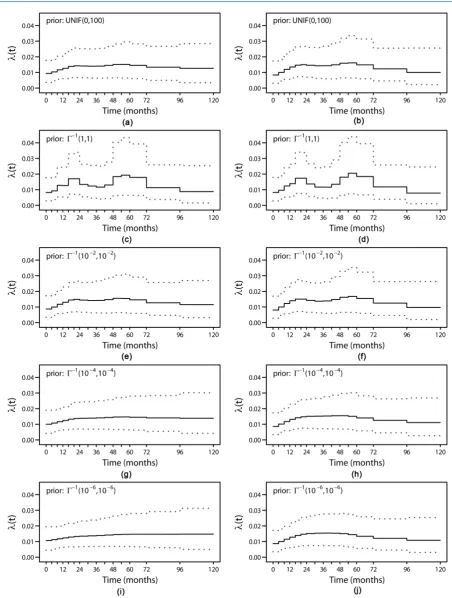
In Figure 3, we reported the estimated hazard function from the ten competing models. Given the PH struc-ture of the model, the shape of the hazard was reported for a fixed set of covariate values: age = 55 years; tumor size = 20 cm; histology = liposarcoma; grading = 2; margin = microscopic. These functions showed distinct be-haviors, thus evidencing the dependency of the results from the choice of the structural components of the model. For what concern the estimates of covariate effects, the values of posterior means and respective credible inter-vals were robust.
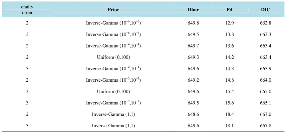
In the following table (Table 2), the competing models have been ranked according to the DIC. Little differ-ences emerged among the models in terms of deviance (Dbar), while major ones were shown in terms of effective degrees of freedom (pD). More interestingly, it seems that the order of the penalty had not a relevant influence on model adequacy, and, thus, the priors had a leading role. Overall, the “best” models correspond to more dif-fuse priors.
4. Discussion
Figure 3. Estimated hazard functions for model (13). Black solid lines: posterior means; dotted lines: 95% credibility inter-vals. Covariate values were: Age: 55 years; tumor size: 20 cm; histology: liposarcoma; grading: 2; margin: microscopic. On the left (panels: a, c, e, g, i) estimates from competing models with a second order difference penalty; on the right (panels: b,
Table 2. Adequacy of the competing models for estimating model (13) Dbar = deviance; pD = effective degrees of freedom;
DIC = Deviance Information Criterion.
enalty
order Prior Dbar Pd DIC
2 Inverse-Gamma (10−6,10−6) 649.8 12.9 662.8
3 Inverse-Gamma (10−6,10−6) 649.5 13.8 663.3
2 Inverse-Gamma (10−4,10−4) 649.7 13.6 663.4
2 Uniform (0,100) 649.3 14.2 663.4
3 Inverse-Gamma (10−4,10−4) 649.6 14.3 663.9
2 Inverse-Gamma (10−2,10−2) 649.2 14.8 664.0
3 Uniform (0,100) 649.6 15.4 665.0
3 Inverse-Gamma (10−2,10−2) 649.5 15.6 665.1
2 Inverse-Gamma (1,1) 648.6 18.4 667.0
3 Inverse-Gamma (1,1) 649.6 18.1 667.8
This is an advantage over frequentist methods, where in the presence of penalties the standard large sample theory does not provide useful results for interval estimation.
Our approach has two main distinctive features with respect to the cited papers on the Bayesian P-splines method:
1) We focused the attention upon on the PE family of models, which did not require specific sampling algo-rithms or specific software for estimation.
2) Due to the link between PE models and the GLM family of regression models, several already available methods, such as the DIC, could be used for developing an efficient strategy of model building. Again, the im-plementation of such methods should not require, in principle, specific accommodations for computation.
The approach has several points in common with Fahrmeir and Hennerfiend’s method ([12]), and, also, with the approach more recently discussed by Murray et al. ([28]). In particular, the family of models considered in our work is a subset of the general model in [12]; however, in our case the likelihood function is tractable, and, thus, specific solutions for approximating the integrated hazard are not needed. Also the model in [28] can be considered as a subset of the general model above, characterized by a piecewise linear hazard function and a tractable likelihood. In the cited paper, the estimates from this model slightly outperformed the PE model in si-mulations, even though for the latter a major robustness of the estimates emerged with sparse data. The major focus of the paper was on the performances of estimates, whereas a formal method of model assessment was not covered.
On the other hand, the major critics to the PE model are (e.g.: [28]): 1) a piecewise constant hazard function is generally not “realistic”; 2) estimates of the hazards are sensitive to the partition of the follow-up time (number and length of intervals). Without any doubt we agree with the first remark. Notwithstanding, we advocate our approach as a useful one for exploratory assessment of the hazard function. In particular, the presence of discon-tinuities in the estimated hazard does not prevent from evidencing relevant features of the “true” hazard. Con-cerning the second critic, this one could not be a real issue. We recall that Eiler’s and Marx’s approach provide a mean for overcoming problems concerning the choice of spline bases and knots, by partitioning the range of the variables in a high number of intervals. However, as far as we know an effective study concerning the issue above has not been carried out yet in our context.
no sensible differences emerged in terms of model adequacy, as indicated by the DIC cri1terion. These results emerged in the estimation of both a “simple” PE model with a smooth hazard function, and in a more complex model including smoothed time-varying effects of a covariate.
Since Bayesian P-splines require the specification of non-informative priors, the sensitivity of posterior esti-mates is an essential task in effective applications. As stated in the method section, the influence of the specific prior for the smoothed parameter has been evidenced in literature, and thus it was one of the primary objects of investigation in our works. For the breast cancer dataset, no relevant influence has been found. We hypothesized that the posterior density “converged” to the (penalized) likelihood function. This was checked by comparing the posterior estimates of all the parameters of the models above with the corresponding estimates obtained by GAM regression (via the mgcv package of R ([37]). We found a good overall agreement between the two me-thods; in particular, the GAM estimates of the hazard function closely overlapped the Bayesian ones.
The low frequency of events occurring at later follow-up times had some influence on the efficiency of the sampling algorithm: in fact, for estimating the model with time-varying coefficients we were forced to truncate the follow-up period to 15 years. However, MCMC diagnostics evidenced no further problems after this. More-over, it is likely that the above scarcity of events affected the accuracy of the estimates of the hazard in the upper tail of the follow-up. Higher or more specific case series are needed for improving the “information content” of such estimates, whatever the specific estimation method or family of regression models adopted in the analysis. Concerning the interpretation of the hazard function, the shape of the hazard resulting in the breast cancer da-ta set was in agreement with clinical knowledge, thus suggesting that the estimation method has a good reliabil-ity in our example.
The application of the method on a relatively small case series (sarcoma dataset) yielded both positive and negative results. Concerning the former ones, the estimates of regression coefficients were robust with respect to the specification of the “structural components” of the regularized PE model (same as above). As emerged in previous work ([16]), this holds also for the estimates of the survival function. The “bad” result consists in the sensitivity of the posterior estimates of the hazard function with respect to the structural components of the model. In this application the prior density for the smoothing parameter was the major determinant of the dif-ferences between the competing models. An interesting result was that the estimates from the “best” model, ac-cording to the DIC criterion, were the most close to the corresponding estimates from GAM regression. This could be a good hint in favor of the utility of the DIC for picking up the best approximation of the underlying hazard; however, a more thorough investigation is needed concerning its effective performances.
5. Conclusions
Our approach provides a practical alternative for regularized estimation of survival regression models. The Gibbs sampling algorithm provides efficient computation of the posterior estimates in the examples reported here. General software routines may be used in real applications, thus facilitating the application of Bayesian P-splines to practitioners. Overall, the estimates are robust with respect to the choice of the components of the smoothing functions included in the model, and provide reliable results. The issue of the sensitivity with respect to the priors results to be limited to the estimates of the hazard function, and seems more only when a relatively small case series are under investigation.
Overall, the proposed method could be a useful tool for the flexible modeling of disease dynamics in complex frameworks like cancer follow-up studies.
Acknowledgements
This work was funded by the Italian Association for Cancer Research (AIRC). IG 2012 rif: 13420, “Statistical Tools for Prognosis and Prediction in Cancer: Assessments and Application to a Sarcoma Case Series”. EMB was Principal Investigator. GM was a fellow of AIRC. The authors thank Dr. Alessandro Gronchi for providing the data on the sarcoma case series.
References
http://dx.doi.org/10.1080/01621459.1992.10476248
[2] Hastie, T. and Tibshirani, R. (1993) Varying-Coefficient Models. Journal of the Royal Statistical Society. Series B
(Methodological), 55, 757-796.
[3] Kooperberg, C., Stone, C.J. and Truong, Y.K. (1995) Hazard Regression. Journal of the American Statistical Associa-tion, 90, 78-94. http://dx.doi.org/10.1080/01621459.1995.10476491
[4] Herndon, J.E. and Harrell, F.E. (1995) The Restricted Cubic Spline as Baseline Hazard in the Proportional Hazards Model with Step Function Time-Dependent Covariables. Statistics in Medicine, 14, 2119-2129.
http://dx.doi.org/10.1002/sim.4780141906
[5] Eilers, P.H. and Marx, B.D. (1996) Flexible Smoothing with B-Splines and Penalties. Statistical Science, 11, 89-102.
http://dx.doi.org/10.1214/ss/1038425655
[6] Kauermann, G. (2005) Penalized Spline Smoothing in Multivariable Survival Models with Varying Coefficients.
Computational Statistics & Data Analysis, 49, 169-186. http://dx.doi.org/10.1016/j.csda.2004.05.006
[7] Ruppert, D., Wand, M.P. and Carroll, R.J. (2009) Semiparametric Regression during 2003-2007. Electronic Journal of Statistics, 3, 1193-1256. http://dx.doi.org/10.1214/09-EJS525
[8] Wood, S.N. (2006) On Confidence Intervals for Generalized Additive Models Based on Penalized Regression Splines.
Australian & New Zealand Journal of Statistics, 48, 445-464. http://dx.doi.org/10.1111/j.1467-842X.2006.00450.x
[9] Wahba, G. (1983) Bayesian “Confidence Intervals” for the Cross-Validated Smoothing Spline. Journal of the Royal Statistical Society. Series B, 45, 133-150.
[10] Silverman, B.W. (1985) Some Aspects of the Spline Smoothing Approach to Non-Parametric Regression Curve Fitting.
Journal of the Royal Statistical Society. Series B, 47, 1-52.
[11] Lang, S. and Brezger, A. (2004) Bayesian P-Splines. Journal of Computational and Graphical Statistics, 13, 183-212.
http://dx.doi.org/10.1198/1061860043010
[12] Fahrmeir, L. and Hennerfiend, A. (2003) Nonparametric Bayesian Hazard Rate Models Based on Penalized Splines Discussion Paper. Sonderforschungsbereich 386 der Ludwig-Maximilians-Universitt Mnchen, No.3 61.
[13] Brezger, A., Kneib, T. and Lang, S. (2005) Bayes X-Software for Bayesian Inference Based on Markov Chain Monte Carlo Simulation Techniques. Journal of Statistical Software, 14.
[14] Boracchi, P., Biganzoli, E.M. and Marubini, E. (2003) Joint Modelling of Cause-Specific Hazard Functions with Cubic Splines: An Application to a Large Series of Breast Cancer Patients. Computational Statistics & Data Analysis, 42, 243-262. http://dx.doi.org/10.1016/S0167-9473(02)00122-6
[15] Boracchi, P., Biganzoli, E.M. and Marubini, E. (2001) Modelling Cause-Specific Hazards with Radial Basis Function Artificial Neural Networks: Application to 2233 Breast Cancer Patients. Statistics in Medicine, 20, 3677-3694.
http://dx.doi.org/10.1002/sim.1112
[16] Marano, G., Boracchi, P. and Biganzoli, E.M. (2014) Estimation of a Piecewise Exponential Model by Bayesian P-Splines Techniques for Prognostic Assessment and Prediction. In: DI Serio, C., Liò, P., Nonis, A. and Tagliaferri, R., Eds., Computational Intelligence Methods for Bioinformatics and Biostatistics, Springer International Publishing, Ge-werbestrasse, 183-198.
[17] Spiegelhalter, D.J., Best, N.G., Carlin, B.P. and Van der Linde, A. (2002) Bayesian Measures of Model Complexity and Fit. Journal of the Royal Statistical Society: Series B (Statistical Methodology), 64, 583-639.
http://dx.doi.org/10.1111/1467-9868.00353
[18] Demicheli, R., Retsky, M.W., Hrushesky, W.J. and Baum, M. (2007) Tumor Dormancy and Surgery-Driven Interrup-tion of Dormancy in Breast Cancer: Learning from Failures. Nature Clinical Practice Oncology, 4, 699-710.
http://dx.doi.org/10.1038/ncponc0999
[19] Demicheli, R., Biganzoli, E.M., Boracchi, P., Greco, M. and Retsky, M.W. (2008) Recurrence Dynamics Does Not Depend on the Recurrence Site. Breast Cancer Research, 10, R83. http://dx.doi.org/10.1186/bcr2152
[20] Rodríguez-Girondo, M., Kneib, T., Cadarso-Suárez, C. and Abu-Assi, E. (2013) Model Building in Nonproportional Hazard Regression. Statistics in Medicine, 32, 5301-5314. http://dx.doi.org/10.1002/sim.5961
[21] Lawless, J.F. (2011) Statistical Models and Methods for Lifetime Data. John Wiley & Sons, Hoboken. [22] Congdon, P. (2007) Bayesian Statistical Modeling. John Wiley & Sons, Hoboken.
[23] DeBoor, C. (1978) A Practical Guide to Splines (Volume 27 of Applied Mathematical Sciences). Revised Edition, Springer-Verlag, New York.
[24] Friedman, J., Hastie, T. and Tibshirani, R. (2001) The Elements of Statistical Learning (Springer Series in Statistics). Springer, Berlin.
Survival Analysis. Springer Science & Business Media, Berlin.
[26] Gelman, A. (2006) Prior Distributions for Variance Parameters in Hierarchical Models. Bayesian Analysis, 1, 515-534. [27] Fahrmeir, L. and Kneib, T. (2009) Propriety of Posteriors in Structured Additive Regression Models: Theory and
Em-pirical Evidence. Journal of Statistical Planning and Inference, 139, 843-859.
http://dx.doi.org/10.1016/j.jspi.2008.05.036
[28] Murray, T.A., Hobbs, B.P., Sargent, D.J. and Carlin, B.P. (2016) Flexible Bayesian Survival Modeling with Semipa-rametric Time-Dependent and Shape-Restricted Covariate Effects. Bayesian Analysis, 11, 381-402.
http://dx.doi.org/10.1214/15-BA954
[29] Thomas, A., Best, N., Lunn, D., Arnold, R. and Spiegelhalter, D. (2004) GeoBUGS User Manual. Medical Research Council Biostatistics Unit, Cambridge.
[30] Kneib, T. and Fahrmeir, L. (2007) A Mixed Model Approach for Geoadditive Hazard Regression. Scandinavian Jour-nal of Statistics, 34, 207-228. http://dx.doi.org/10.1111/j.1467-9469.2006.00524.x
[31] Ardoino, I., Miceli, R., Berselli, M., Mariani, L., Biganzoli, E.M., Fiore, M., Colini, P., Stacchiotti, S., Casali, P.G. and Gronchi, A. (2010) Histology-Specific Nomogram for Primary Retroperitoneal Soft Tissue Sarcoma. Cancer, 116, 2429-2436. http://dx.doi.org/10.1002/cncr.25057
[32] Veronesi, U., Marubini, E., Del Vecchio, M., Manzari, A., Andreola, S., Greco, M., Luini, A., Merson, M., Saccozzi, R., Rilke, F. and Salvadori, B. (1995) Local Recurrences and Distant Metastases after Conservative Breast Cancer Treatments: Partly Independent Events. Journal of the National Cancer Institute, 87, 19-27.
http://dx.doi.org/10.1093/jnci/87.1.19
[33] R Core Team (2013) R: A Language and Environment for Statistical Computing. R Foundation for Statistical Compu-ting, Vienna. http://www.R-project.org/
[34] Sturtz, S., Ligges, U. and Gelman, A. (2005) R2WinBUGS: A Package for Running WinBUGS from R. Journal of Statistical Software, 12, 1-16. http://dx.doi.org/10.18637/jss.v012.i03
[35] Plummer, M., Best, N., Cowles, K. and Vines, K. (2006) CODA: Convergence Diagnosis and Output Analysis for MCMC. R News, 6, 7-11.
[36] Gray, R.J. (1996) Hazard Rate Regression Using Ordinary Nonparametric Regression Smoother. Journal of Computa-tional and Graphical Statistics, 5, 190-207.
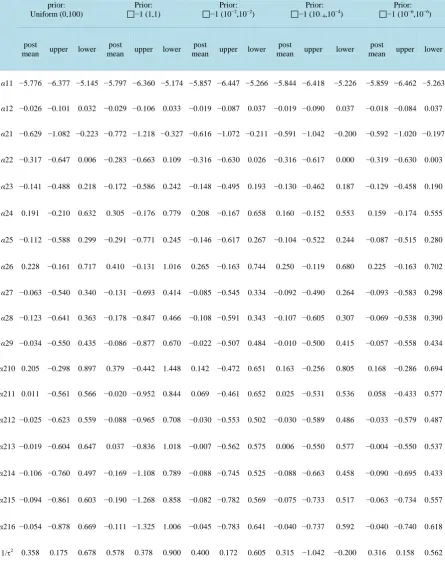
Appendix 1
Table A1. Estimates for application 1: Posterior means and 95% credible intervals (a) hazard parameters, second order
dif-ference penalty. (b) Regression coefficients, second order difdif-ference penalty.
(a)
prior: Uniform (0,100)
Prior:
−1 (1,1) −1 (10Prior: −2,10−2) −1 (10Prior: −4,10−4)
Prior:
−1 (10−6,10−6)
post
mean upper lower post
mean upper lower post
mean upper lower post
mean upper lower post
mean upper lower
α11 −5.776 −6.377 −5.145 −5.797 −6.360 −5.174 −5.857 −6.447 −5.266 −5.844 −6.418 −5.226 −5.859 −6.462 −5.263
α12 −0.026 −0.101 0.032 −0.029 −0.106 0.033 −0.019 −0.087 0.037 −0.019 −0.090 0.037 −0.018 −0.084 0.037
α21 −0.629 −1.082 −0.223 −0.772 −1.218 −0.327 −0.616 −1.072 −0.211 −0.591 −1.042 −0.200 −0.592 −1.020 −0.197
α22 −0.317 −0.647 0.006 −0.283 −0.663 0.109 −0.316 −0.630 0.026 −0.316 −0.617 0.000 −0.319 −0.630 0.003
α23 −0.141 −0.488 0.218 −0.172 −0.586 0.242 −0.148 −0.495 0.193 −0.130 −0.462 0.187 −0.129 −0.458 0.190
α24 0.191 −0.210 0.632 0.305 −0.176 0.779 0.208 −0.167 0.658 0.160 −0.152 0.553 0.159 −0.174 0.555
α25 −0.112 −0.588 0.299 −0.291 −0.771 0.245 −0.146 −0.617 0.267 −0.104 −0.522 0.244 −0.087 −0.515 0.280
α26 0.228 −0.161 0.717 0.410 −0.131 1.016 0.265 −0.163 0.744 0.250 −0.119 0.680 0.225 −0.163 0.702
α27 −0.063 −0.540 0.340 −0.131 −0.693 0.414 −0.085 −0.545 0.334 −0.092 −0.490 0.264 −0.093 −0.583 0.298
α28 −0.123 −0.641 0.363 −0.178 −0.847 0.466 −0.108 −0.591 0.343 −0.107 −0.605 0.307 −0.069 −0.538 0.390
α29 −0.034 −0.550 0.435 −0.086 −0.877 0.670 −0.022 −0.507 0.484 −0.010 −0.500 0.415 −0.057 −0.558 0.434
α210 0.205 −0.298 0.897 0.379 −0.442 1.448 0.142 −0.472 0.651 0.163 −0.256 0.805 0.168 −0.286 0.694
α211 0.011 −0.561 0.566 −0.020 −0.952 0.844 0.069 −0.461 0.652 0.025 −0.531 0.536 0.058 −0.433 0.577
α212 −0.025 −0.623 0.559 −0.088 −0.965 0.708 −0.030 −0.553 0.502 −0.030 −0.589 0.486 −0.033 −0.579 0.487
α213 −0.019 −0.604 0.647 0.037 −0.836 1.018 −0.007 −0.562 0.575 0.006 −0.550 0.577 −0.004 −0.550 0.537
α214 −0.106 −0.760 0.497 −0.169 −1.108 0.789 −0.088 −0.745 0.525 −0.088 −0.663 0.458 −0.090 −0.695 0.433
α215 −0.094 −0.861 0.603 −0.190 −1.268 0.858 −0.082 −0.782 0.569 −0.075 −0.733 0.517 −0.063 −0.734 0.557
α216 −0.054 −0.878 0.669 −0.111 −1.325 1.006 −0.045 −0.783 0.641 −0.040 −0.737 0.592 −0.040 −0.740 0.618
(b)
Prior: Uniform (0,100)
Prior:
Γ-1(1,1)
Prior:
Γ-1(10−2,10−2)
Prior:
Γ-1(10−4,10−4)
Prior:
Γ-1(10−6,10−6)
post
mean upper lower post
mean upper lower post
mean upper lower post
mean upper lower post
mean upper lower
β1 −0.550 −0.829 −0.252 −0.533 −0.814 −0.242 −0.538 −0.816 −0.235 −0.541 −0.842 −0.233 −0.537 −0.827 −0.248
β2 −0.671 −0.957 −0.379 −0.656 −0.931 −0.373 −0.660 −0.934 −0.355 −0.666 −0.956 −0.365 −0.660 −0.939 −0.369
β3 −0.397 −0.704 −0.098 −0.384 −0.692 −0.080 −0.387 −0.678 −0.086 −0.390 −0.687 −0.080 −0.388 −0.669 −0.090
β4 −0.363 −0.704 −0.001 −0.351 −0.703 0.003 −0.353 −0.691 −0.004 −0.355 −0.719 0.009 −0.353 −0.682 −0.011
β5 0.530 0.126 0.975 0.551 0.162 0.960 0.562 0.172 1.005 0.556 0.166 0.954 0.556 0.166 0.986
β6 0.637 0.242 1.064 0.654 0.259 1.064 0.665 0.273 1.095 0.659 0.262 1.062 0.660 0.265 1.085
β7 0.845 0.431 1.280 0.862 0.458 1.275 0.878 0.488 1.306 0.870 0.486 1.281 0.871 0.470 1.300
β8 1.167 0.731 1.619 1.185 0.761 1.625 1.197 0.767 1.677 1.190 0.785 1.627 1.193 0.764 1.650
β9 −0.037 −0.256 0.183 −0.041 −0.265 0.179 −0.039 −0.259 0.175 −0.039 −0.260 0.185 −0.038 −0.265 0.180
β10 0.208 −0.041 0.444 0.204 −0.052 0.442 0.210 −0.035 0.443 0.211 −0.051 0.459 0.208 −0.048 0.442
β12 0.885 0.651 1.106 0.888 0.662 1.101 0.884 0.665 1.104 0.884 0.657 1.109 0.892 0.663 1.118
β13 0.145 −0.015 0.301 0.148 −0.009 0.313 0.146 −0.019 0.305 0.144 −0.015 0.302 0.148 −0.014 0.309