Approximation Effects Due to Diffuse Derivatives from Polynomial Basis

(1)

International Journal of Emerging Technology and Advanced Engineering

Website: www.ijetae.com (ISSN 2250-2459,ISO 9001:2008 Certified Journal, Volume 3, Issue 7, July 2013)

415

Approximation Effects Due to Diffuse Derivatives from

Polynomial Basis

Geethu S. Pillai

1

, K.A. Narayanankutty

2

, K.P. Soman

3

1

M.Tech, Final Year Student, Department of CEN, Amrita Vishwa Vidyapeetham, Coimbatore

2_{Professor, Department of ECE, Amrita Vishwa Vidyapeetham, Coimbatore}

3_{Professor and Head, Department of CEN, Amrita Vishwa Vidyapeetham, Coimbatore}

Abstract—Moving Least Squares(MLS) is a method of reconstructing functions that are continuous from a group of random point samples through the calculation of a weighted least squares measure. At instances in Moving Least Squares (MLS), we slash out some of the terms of classical derivatives to get smaller expressions which are called the diffuse derivatives. In this paper, we construct a polynomial basis from which the diffused derivatives are obtained. Finally, a three dimensional object is constructed from a two dimensional image. A shape function is created along with its first and second derivatives and the diffuse derivatives, in order to observe the changes that are taking place in the object.

Keywords— Mesh free methods; weighted least squares; moving least squares approximation (MLS); classical derivatives; diffuse derivatives

I. INTRODUCTION

Meshes are a network of nodes that are interconnected to one another. The classes of numerical methods that have unique advantages over the existing mesh-based methods are the mesh-less or the mesh-free methods. Unlike, the mesh based techniques; here instead of the estimation of solution of physical equations on a mesh structure, a solution is desired on a group of nodes. Meshfree methods uses a set of nodes scattered within the problem space as well as sets of nodes scattered on the boundaries. The main objective of mesh-less methods is to eliminate a part of the structure by building up the approximation in terms of nodes as in [2]. The term ―mesh less‖ suggests that it is free from the mesh. In this category, a mesh will not be present which leads to the independence of the nodes. In the meshfree methods moving discontinuities can be well handled without re-meshing with minimum costs in the mortification of accuracy that leads to the solution of problems that cannot be solved conveniently with the mesh based methods. Eventhough the origination of the meshless or meshfree methods occurred twenty years ago, it was only recently that the efforts for researches were devoted.

The advantages of mesh-free methods over the mesh methods is that, firstly, mesh free techniques consumes lesser time compared to mesh based methods. Secondly, since the nodes or points are independent to each other, the cost is reduced. The process of re-meshing is quite expensive and the projection between the meshes which are successive leads to degradation of accuracy which in turn results in the increase in computational cost. These unique features increase the range of problems that can be addressed by the mesh free methods rather than the mesh based techniques. Another major advantage of the mesh free method is that these can handle large deformations more robustly. The MLS approximation method approximates value u(x) of unknown function u from the given data. Mathematically we can express this as

1

ˆ( )

( ) (

)

( )

N

j p

j

p y

a y p y

p y







Where

a y

_j

( )

are called the shape functions, which is the major ingredient in this paper. Based on these shape functions, the derivatives are estimated. In this paper, the concept of the Moving Least Squares is applied along with the concept of the diffuse derivatives. The concept of diffuse derivatives, introduced in [11] undergoes a direct estimation of the derivatives

D u x



( )

from the given data

1

( ),..., (

_n

)

u x

in this paper. This is in turn linked to the concepts of diffuse derivatives. As in [8], consider an unknown function p with nodes

y

₁

,...,

y

_N having data

p y

( ),..., (

₁

p y

_N

)

.

(2)

International Journal of Emerging Technology and Advanced Engineering

416

In the coming section, 2, a detailed explanation on the MLS methodology along with the derivation of shape function and its corresponding derivatives has been provided. An explanation of diffuse derivatives is provided in the section 3.

II. MOVING LEAST SQUARES

The approximation method called MLS Approximation is actually an alternative to the radial basis function approximation. This real valued function depends on the distance from the origin alone. Before going to the moving least squares, let’s see a gist of exactly what a weighted least square(WLS) is. In the WLS functional, each of the squared terms used in a traditional least squares minimization is multiplied by a corresponding weight function. Thus, it can be inferred that each of these squared terms is highly affected or influenced by its respective weights. Mathematically, the weighted least squares functional can be expressed as





2

1

1 ( )

(

)

2

n

T

a a a

a

J g

w

p

x g

u







In order to approximate multidimensional surfaces, we introduced the MLS approximation. In the MLS method, the approximation of a function is obtained by the solution of many small linear systems, rather than solving a single linear system. In the weighted least squares functional, for each point x, the corresponding

w

_a is calculated. Then the functional J is minimized with respect to each of the

g

_i. The minimization procedure will be repeated, for each time there is a movement to a new point. Thus this method is named as the MLS method, since it depends on the current point x. Several equivalent formulations exist for the MLS approximation scheme.

In the paper [24], it has been well explained that MLS surfaces can be represented as a smooth surface from the given point cloud data.

Consider a three dimensional domain as in [24] with a discrete point set

P





p

_i



R

D



,

i





1, 2,...,

n



where

i

p

is the nodal data that was sampled from an unknown surface, say S. The main goal of MLS is to directly define a reconstructed surface from the given discrete set of points P.

Now, let’s consider a surface function f(x) that is defined over an arbitrary space



, that approximates the given values f_i for a moving point

x



R

D.

Now let’s start this with the process of applying the WLS, f (x)' for a fixed point in the three dimensional domain. Then, this point is to be moved through the entire domain, where the WLS is to be calculated for each point individually.

Then the function f(x) is obtained from a set of local approximation functions f’(x).





'

1

( )

arg min

(

)

n

i i i i

i

f x

w

x

p

f

p

f







'

[1, ]

( )

T

( )

_j

( )

_j

( )

j m

f x



g

x c x







_

g x c x



Therefore,





2

( )

min

i i T

(

i

) ( )

i i

f x





w

x



p

g

p c x



f

Where the polynomial basis vector is



1 2



( )

( ),

( ),...,

_m

( )

T

g x



g x g x

g

x



1 2



( )

( ),

( ),...,

_m

( )

T

c x



c x c x

c

x

be the vector of unknown coefficients and

w

_i



x



p

_i



be the weighting function to the moving point x.

The weighting function has certain advantages such as compact support, they are non negative.

A. Derivation of MLS Shape Function and its Derivatives[14]

As in [14], consider, finding the approximate solution,

( )

h

u x

of

u

_a at points

x

_a. According to the least squares

minimization, our objective is

2

(

)

h

a a

u x

u











. Assume

choosing a polynomial expression as in [14] such that,

u x

h

( )



g

₁



g x

₂



g x

₃



...

g

m₁

x

m (1)

(3)

International Journal of Emerging Technology and Advanced Engineering

417





1 2 3 2 1

( )

1 ...

.

h T m

m

g

u x

p

x g

x x

x

g

_









_

_







(2)

Using equation (2), the least squares functional can be written as





2 1

1 (

)

2

n h a a a

J

u x

u







(3)





2

1

1 (

)

2

n T a a a

J

p

x g

u







(4)

1/2 is added for convenience.

MLS shape functions have the property of compact support, which means that the support will be constrained to a small region around a particular node. Since the MLS shape functions have the property of compact support, local solution will be affected by the local nodes alone and that the far away nodes have no influence. Hence each summation term in the least square function that is indexed by a, is weighted by a weight function

w

_a, so that the terms influence will be constrained to node a and the surrounding nodes.

Based on this intuition, equation (4) is modified by adding a weighted term

w

_a.

1 (

)

(

)

2

T

J



Pg



u W Pg



u

(5)

It is now necessary to minimize the least square functional with respect to each

_gi

. Before performing the minimization, the functional must be expressed in terms of matrix.

1 (

)

(

)

2

T

J



Pg



u W Pg



u

(6)

Where

1 1 2 1 1

1 2

( )

.

( )

.

(

)

(

)

(

)

k

n n k n

p x

P

p x



































(7)

The size of the matrix P is n by k.

W is a n by n matrix whose diagonal elements are weights of corresponding points.

1 1

2 2

(

)

0 (

)

.

0

_n

(

_n

)

w x x

W

w x x









_























_







(8)

Vector g is k by 1 and vector u is n by 1.

Setting,

J

0 g



_



(

Pg



u WP

)

T



0

(9) Transposing equation 9, we get,

(

WP

) (

T

Pg



u

)



0

(10)

0

T T

P WPg



P Wu



Multiplying throughout,

P WPg

T



P Wu

T

(11)

From equation (11), we can infer that

T

A



P WP

T

B



P W

Thus, equation (11) becomes,

Ag



Bu

(12)

Solving for the coefficient that is unknown 1

(4)

International Journal of Emerging Technology and Advanced Engineering

418

Substituting equation (13) in equation (2), we get

( )

h T

u



p

x g

(14)



p

T

( )

x A Bu

1 (15)

Mathematically, the approximation can be expressed as:

1

n

h T

a a

a

u



  





(16)

Comparing equations (15) and (16), 1

( )

T T

f



p

x A B

 (17)

To derive the first derivative of the shape function,



, with respect to the kth dimension



_,T_k

( )

x



p A B

_,T_k 1



p A B

T _,_k1



p A B

T 1 _,_k (18)

with

A

_,_k1

 

A A A

1 _,_k 1

Taking the derivative of (12), we get

,k ,k ,k

A g



Ag



B u

(19) Solving equation (19),

1 1 1

,k ,k ,k

g



A B u



A A A Bu

  (20)

Estimate the derivative of equation (13),

g

_,_k



A B u

1 _,_k



A Bu

_,_k1 (21)

From the above two equations, (20) and (21), we can infer that since both the equations are same expect for the Bu term, we can equate them.

A

_,_k1

 

A A A

1 _,_k 1 (22)

Similarly, the second derivatives can be estimated by taking the derivative of equation (18) with respect to the lth dimension.

III. DIFFUSE DERIVATIVES

In the paper [23], the authors explained a new approximation methodology called the ―diffuse approximation‖ method. The diffuse approximation method is actually a generalized form of the Finite Element Method. Certain limitations of the Finite Element approximation were eradicated using this technique.

This newly introduced approximation method may be used for developing smooth approximations as well as for the accurate estimation of the derivatives. This methodology is used in estimating the numerical solutions of the PDE’s. Thus, they were named as the ―Diffuse Element Method‖ that acquires certain merits compared to the classical FEM method.

The main aim of the MLS approach is to acquire an approximation with a great accuracy level in the bounded domain that is similar to the SPH technique. The paper [24] also gives a proper definition for the diffuse derivatives. The approximation of each of the derivatives of u in each direction, is the respective derivative of u , i.e., p

f

_I



a

₀



a x

₁ _I



a x

₂ _I2

 

...

a x

_k _Ik

The second term on the right side of the above equation is not trivial. In order to estimate the derivatives of the coefficients, c, the linear equations must be resolved using matrix M, which is an expensive task. Also, to compute the derivatives of the coefficients, a prior knowledge about the particles surrounding each of the points must be known whereas, the estimation of the derivatives of the polynomials, which is the first term in the above formulation, can be easily evaluated. Here, the derivatives can be estimated without knowing about the particles surrounding the point.

Two scientists namely, Villon and Nayroles et.al [23] in 1992, introduced the concept of the diffuse derivatives which included the latter methodology, i.e., approximating the derivatives of the polynomials.

( )

P

P T T

z x z x

u

P

c x

x

z

x



_ _







It can be inferred that the computation of the derivatives of shape functions needed an extra cost.

IV. PROPOSED SYSTEM

(5)

International Journal of Emerging Technology and Advanced Engineering

419

The concept of diffuse derivatives undergoes a direct estimation of the derivatives

D u x



( )

from the given data

1

( ),..., (

_n

)

u x

as given in paper [1]. Here, it is necessary to get the derivatives of polynomials. We have an order upto degree m. So, all the polynomials of degree upto m are reproduced for all the choices of weights, wherein the full and the diffuse derivatives of these polynomials coincide. For setting the linear system, use of

ˆ

u

and its derivatives is not needed. After solving the system, the values

u x

ˆ( )

_j will have its approximations at the nodes. Once, the processing is done, it is necessary to estimate exact derivatives or the diffuse derivatives of the solution that has been approximated. This is in turn linked to the concepts of diffuse derivatives. This methodology is then applied to the image. Also, this method provides a smooth approximation using the set of nodes, rather than the classical FEM methodology.

V. RESULTS AND DISCUSSIONS

[image:5.612.328.564.223.395.2]

The algorithm presented in this paper was successfully implemented to construct a three dimensional object projected from a two dimensional image. Then, we applied the shape function, phi, to this image, which did not bring out much of a difference. In order to check the efficiency of the algorithm, we analyzed the same for different orders of the polynomial basis, m. Figure (1) shows the original constructed three dimensional images on the 2D plane.

FIGURE 1. Original Image

Initially, we tested for different orders of the shape function, phi, but there was no change that could be analyzed.

To create the matrix of the MLS shape function, we introduce a variable, delta, which is the size of support of the MLS weight function. This means that their support is limited to a small region around a particular node. Here, we assume that the delta value is directly proportional to the maximum distance between all nodes scattered in the domain.

delta

 

c h

c

 

2 m

delta

  

2 m h

[image:5.612.65.274.483.659.2]

FIGURE 2. Shape function when the order, m=1

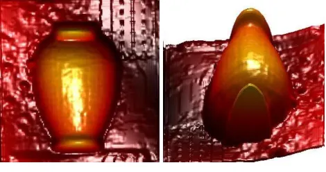
But when we performed the first derivatives of the MLS shape functions to the image, variations were estimated given in the figure 3, which depicts that after each order the deformation in the image increases. The image obtained when the order is 2 will be facing more deformation than the first order

.

FIGURE 3. First derivatives applied when m=2

[image:5.612.327.562.502.626.2]

(6)

International Journal of Emerging Technology and Advanced Engineering

420 FIGURE 4. First diffuse derivatives for m=3 and delta=1.5

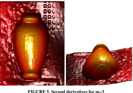
[image:6.612.55.282.133.257.2]

The following figures 5 and 6 shows the changes transpired for the image when we apply the second derivatives and the second diffuse derivatives. But it can be inferred from the figure 6 that when the second diffuse derivatives is applied to the image, the image has no change and it is similar to that of the original image.

FIGURE 5. Second derivatives for m=3

It could be observed that the three dimensional object that we finally received was smoother and more efficient. The approximation of the diffuse derivatives from the polynomial basis led to a good convergence.

In this paper, we investigated the change in the image in the cases of the shape function, first and second derivatives and diffuse derivatives. Also, the final result could be changed by changing the values of the support domain delta to adjust the discontinuities.

FIGURE 6. Second diffuse derivatives for m=3

It can be discovered that, when we change the value of delta, the way in which the image changes also varies.

VI. CONCLUSION

This algorithm was successfully and steadily implemented on an image creating a three dimensional object without any loss of efficiency and accuracy.

Also, the application of diffuse derivatives along with the MLS helped us to provide a smooth approximation using the set of nodes. In this paper, we investigated the change in the image in the cases of the shape function, first and second derivatives and diffuse derivatives. We constructed a polynomial basis from which the diffused derivatives are obtained. The mesh-free shape function has more smoothness. The shape function phi and the second diffuse derivatives showed no change in the original image. An analysis was carried out to study the change in the image by changing the delta value and the discontinuities could be well analyzed. The use of full derivatives alone will be more expensive.

Acknowledgement

The first author would like to thank Dr.P.Geetha and Ms.Sowmya for their suggestions during the reviews and encouragement.

REFERENCES

[image:6.612.52.286.353.516.2]

(7)

International Journal of Emerging Technology and Advanced Engineering

421

[2] T. Belytschko, Y. Krongauz, D.Organ, M. Fleming, P. Krysl, Meshless methods: An overview and recent developments, ―Computer Methods in Applied Mechanics and Engineering‖, Volume 139, Issues 1–4, 15 December 1996, pp. 3–47.

[3] Stephen Beissel; Ted Belytschko , Nodal integration of the element-free Galerkin method, ‖Computer Methods in Applied Mechanics and Engineering‖. 1996; 139(1-4): pp.49-74

[4] Cingoski, V. ; Miyamoto, N. ; Yamashita, H., Element-free Galerkin method for electromagnetic field computations , IEEE Explorer, Volume: 34 , Issue: 5 , Part: 1, 1998 , pp. 3236 – 3239

[5] Atluri, S. N.; Zhu, T., A new Meshless Local Petrov-Galerkin (MLPG) approach in computational mechanics, ― Computational Mechanics‖, Volume 22, Issue 2, pp.117-127 (1998)

[6] Mehdi Dehghan, Davoud Mirzaei, Meshless Local Petrov–Galerkin (MLPG) method for the unsteady magnetohydrodynamic (MHD) flow through pipe with arbitrary wall conductivity, ―Applied Numerical Mathematics‖, Volume 59, Issue 5, May 2009, Pages 1043–1058

[7] T.P. Fries, H.G. Matthies: Classification and overview of meshfree methods, Informatikbericht-Nr. 2003-03, Technische Universität Braunschweig, Braunschweig, 2003

[8] Davoud Mirzaei, Recent developments in MLS based mesh less methods,― Second khansar conference on mathematical sciences, 4th

conference on numerical analysis and its applications‖, Iran, May 7-8, 2013

[9] T.Belytschko, Y. Krongauz, D. Organ, M. Fleming, P.Krysl, Meshless methods:An overview and recent developments, 1996 computer methods in applied mechanics and engineering, Vol 139, pp 3-47

[10] Nguyen V.P., Rabezuk T., Bordas S., Duflot M. (2008): ― Meshless methods: A review and computer implementation aspects, ‖ Mathematics and computers in simulation, vol. 79, pp. 763-813. [11] B. Nayroles, G. Touzot, P. Villon, Generalizing the finite element

method: Diffuse approximation and diffuse elements, Computational Mechanics - COMPUTATION MECH , vol. 10, no. 5, pp. 307-318, 1992.

[12] Antonio Huerta, Ted Belytschko, Sonia Fernandez-Mendez, Timon Rabezuk,; Meshfree Methods, ―Encyclopedia of computational mechanics‖, 2004

[13] P.Lancaster and K.Salkauskas, Surfaces generated by moving least squares, ―Mathematics of Computation‖, volume 37, number 155, July 1981.

[14] Louie L. Yaw, Introduction to Moving Least Squares(MLS) Shape Functions, April 19 2009,

[15] P. Breitkopf, A. Rassineux, G. Touzot, and P. Villon. Explicit form and effcient computation of MLS shape functions and their derivatives. Int. J. Numer. Methods Eng., 48:451-466, 2000. [16] R. Franke. Scattered data interpolation: tests of some methods.

Mathematics of Computation, 48:181-200, 1982.

[17] D. Shepard. A two-dimensional interpolation function for irregularly-spaced data. In Proceedings of the 23th National Conference ACM, 1968 pp.517-523.

[18] H. Wendland. Local polynomial reproduction and moving least squares approximation. IMA J. Numer. Anal., 21:285{300, 2001. [19] B. Nyroles, G. Touzot, and P. Villon. Generalizing the fnite element

method: Diffuse approximation and diffuse elements. Comput. Mech., 10:307{318, 1992.

[20] D. Levin. The approximation power of moving least-squares. Math. Comput., 67:1517-1531, 1998.

[21] Gregory E. Fasshauer, Meshfree Approximation Methods with Matlab, Interdisciplinary Mathematical Sciences- Vol 6. 2007 [22] Z-Q. Cheng, Y-Z Wang, B. Li, K. Xu, G. Dang and S-Y. Jin, A

survey of methods for moving least squares surfaces, IEEE/EG Symposium on Volume and Point-Based Graphics (2008).

[23] B. Nayroles, G. Touzot and P. Villon; Generalizing Finite Element: Diffuse approximation and Diffuse Elements, computational mechanics(1992)10, pp.307-318