The development of a fixed wing aircraft analysis and design flight dynamic software

(1)

iii

THE DEVELOPMENT OF A FIXED WING AIRCRAFT ANALYSIS AND DESIGN FLIGHT DYNAMIC SOFTWARE

AHMAD ESHTIWEY AHMAD ALAIAN

A thesis submitted in 18 / 02 / 2016

fulfillment of the requirement for the award of the

Doctor of Philosophy in Mechanical and Manufacturing Engineering

Faculty of Mechanical and Manufacturing Engineering Universiti Tun Hussien Onn Malaysia

(2)

v

ACKNOWLEDGEMENT

This research thesis was made possible through the enormous help and great support from everyone, including: my father, mother, wife, teachers and family. I would like to dedicate my acknowledgment of gratitude toward the following significant advisors and contributors:

First and foremost, I would like to thank Ir. Dr. Bambang Basuno for his endless support and encouragement. He kindly read my paper and offered invaluable detailed advices on grammar, organization, and the theme of the thesis.

Second, I would like to thank Assoc Prof. Dr. Zamri Bin Omar who read my thesis and he provided me with valuable feedbacks and advice. In addition I would like to thank all the other professors who have taught me about Mechanical Engineering and Manufacturing in general and Aeronautics department in particular and helped me to gain my doctoral degree.

(3)

vi

ABSTRACT

(4)

vii

(5)

viii

ABSTRAK

(6)

ix

(7)

x

CONTENTS

TITLE iii

ACKNOWLEDGEMENTS v

ABSTRACT vi

CONTENTS x

LIST OF FIGURES xiv

LIST OF TABLES xxii

LIST OF SYMBOLS xxv

LIST OF APPENDIXES xxvii

CHAPTER 1 INTRODUCTION 1

1.1 Background of study 1

1.2 Problem statement 4

1.3 Objectives 5

1.4 Scope of work 6

1.5 Research methodology 9

1.6 The results of the research work 9

1.7 Organization of the thesis 10

CHAPTER 2 LITERATURE REVIEW 12

2.1 Aircraft flight dynamics 12

2.2 The governing equation of flight motions 15 2.3 Simplified forms of the governing equation of

flight motion 25

2.3.1 Simplified longitudinal direction

form of equations 26

(8)

xi

equations 29

2.4 The trim condition governing equation 30

2.5 Flying and handing qualities 33

2.5.1 Longitudinal flying qualities 34

2.5.1.1Static response 34

2.5.1.2Phugoid response 34

2.5.1.3Short period response 34

2.5.2 Lateral flying qualities 35

2.5.2.1Rolling motion 35

2.5.2.2Spiral stability 36

2.5.2.3Lateral directional oscillations-Dutch

roll 37

2.6 Compression between linear and non-linear

equation 37

2.7 An overview of the solution of the

governing equation for flight motion 38

2.7.1 Euler’s method 40

2.7.2 The second order Runge-Kutta method 41 2.7.3 The fourth order Runge-Kutta method 41 2.7.4 Adams-Bashforth method of order

three 41

2.8 An overview on the manner of controlling

the aircraft movement 42

2.9 Aircraft controller design 44

2.10 The flight dynamics software 46

2.11 The flight dynamics software development in

the past 48

CHAPTER 3 METHODOLOGY 51

3.1 Introduction 51

3.2 The aerodynamics characteristics estimation 52 3.3 The aircraft dimensional stability and control

derivatives 57

(9)

xii

motion 59

3.4.1 The solution of flight motion based on

state-space approach 59

3.4.2 The solution of flight motion based on

transfer functions approach 62

3.5 The classical PID control design estimation 70 3.5.1 The basic idea of the control system

design 72

3.5.2 The technique in developing PID

controller 76

3.6 Non-linear simulation aircraft behaviour 80

CHAPTER 4 RESULTS AND DISCUSSION 82

4.1 Introduction 82

4.2 Longitudinal and lateral directional dynamic

stability behaviours 82

4.2.1 Input data 85

4.2.2 The output and the results of the longitudinal and lateral directional

dynamic stability behaviours 88 4.2.2.1The stability derivatives of longitudinal

and lateral directions 88

4.2.2.2The solution for flight motion 89 4.2.3 Time history and stability behavior of

aircrafts 97

4.2.3.1Time history or stability behavior in the

longitudinal direction 100

4.2.3.2Time history and stability behavior in

the lateral direction 111

4.3 Controller design 138

4.3.1 The results of Cessna 182 controller

design 140

4.3.1.1The longitudinal direction controller

(10)

xiii

4.3.1.2The lateral direction controller design 142 4.3.2 Time history of Cessna 182 aircraft 152 4.3.2.1Time history of pitch angle controller 153 4.3.2.2Time history of roll angle controller 158 4.3.2.3Time history of yaw angle controller 168 4.4 The non-linear simulation aircraft behaviour 182

4.4.1 The geometry and the overall performance data of Piper Cherokee PA

28-161 Warrior 182

4.4.2 The evaluation of the aerodynamics characteristics of the Piper Cherokee

PA 28-161 188

4.4.3 The Simulink diagram for the Piper

Cherokee PA 28-161 191

4.4.4 The estimation of flight dynamics

behavior with Simulink 194

4.4.5 Comparison between non-linear and

linear models 209

4.5 Summary 214

CHAPTER 5 CONCLUSION AND FUTURE WORK 217

5.1 Introduction 217

5.2 Conclusion 217

5.3 Contribution and the novelty of research 218

5.4 Future work 219

REFERENCES 221

(11)

xiv

LIST OF FIGURES

1.1 The automatic and the manual flight control loops 3 1.2 Flight dynamics analysis and design procedure 7 2.1 The locations of the origin of the coordinate systems 16 2.2 The orientation of body axis, stability axis, and wind

axis 18

2.3 Body axis coordinate system 18

2.4a Definitions of aerodynamic forces, thrust, and

acceleration gravitation in body axis coordinate 19 2.4b Definitions of moments, linear, and angular velocity

in body axis coordinate system 19

2.5 Flowchart for non-linear simulation steps 40

2.6 The conventional aircraft 43

2.7 Unity feedback system 45

3.1 A simplified body diagram of the mass, spring and

damper 73

3.2 The block diagram of the vehicle as an open loop

system 73

3.3 The displacement response of mass, spring and damper as an open loop system due to a unit step

function 74

3.4 The control system with a unity feedback 75 3.5 The displacement response of mass, spring and

damper as a closed-loop system due to a unit step

function 75

(12)

xv

equation and PID controller 77

3.7 The step response of Method I controller approach 78 3.8 The step response of Method II controller approach 79 3.9 The step response of PID SISO controller approach 79 4.1 Two types of propeller driven aircrafts 84

4.2 Two types of turbo driven aircrafts 84

4.3 MATLAB start menu for the direction analysis 84 4.4 MATLAB start menu for the aircraft model analysis 85 4.5a MATLAB start menu for longitudinal direction 99 4.5b MATLAB start menu to select the lateral effect

control surfaces 99

4.6a Longitudinal direction responses following elevator

single doublet impulse maneuvers of Cessna 182 100 4.6b Longitudinal direction responses following elevator

single doublet impulse maneuvers of Cessna 310 101 4.6c Longitudinal direction responses following elevator

single doublet impulse maneuvers of Learjet 24 101 4.6d Longitudinal direction responses following elevator

single doublet impulse maneuvers of Cessna 620 102 4.7a Longitudinal direction responses following elevator

multiple doublets impulse maneuvers of Cessna 182 103 4.7b Longitudinal direction responses following elevator

multiple doublets impulse maneuvers of Cessna 310 104 4.7c Longitudinal direction responses following elevator

multiple doublets impulse maneuvers of Learjet 24 105 4.7d Longitudinal direction responses following elevator

multiple doublets impulse maneuvers of Cessna 620 105 4.8a Longitudinal direction responses following elevator

single doublet maneuvers of Cessna 182 106 4.8b Longitudinal direction responses following elevator

single doublet maneuvers of Cessna 310 106 4.8c Longitudinal direction responses following elevator

(13)

xvi

4.8d Longitudinal direction responses following elevator

single doublet maneuvers of Cessna 620 107 4.9a Longitudinal direction responses following elevator

multiple doublets maneuvers of Cessna 182 108 4.9b Longitudinal direction responses following elevator

multiple doublets maneuvers of Cessna 310 108 4.9c Longitudinal direction responses following elevator

multiple doublets maneuvers of Learjet 24 109 4.9d Longitudinal direction responses following elevator

multiple doublets maneuvers of Cessna 620 109 4.10a Lateral direction responses following aileron single

duplet impulse maneuvers of Cessna 182 112 4.10b Lateral direction responses following aileron single

duplet impulse maneuvers of Cessna 310 112 4.10c Lateral direction responses following aileron single

duplet impulse maneuvers of Learjet 24 113 4.10d Lateral direction responses following aileron single

duplet impulse maneuvers of Cessna 620 113 4.11a Figure 4.11a: Lateral direction responses following

aileron multiple doublets impulse maneuvers of

Cessna 180 115

4.11b Lateral direction responses following aileron multiple

doublets impulse maneuvers of Cessna 310 115 4.11c Lateral direction responses following aileron multiple

doublets impulse maneuvers of Learjet 24 116 4.11d Lateral direction responses following aileron multiple

doublets impulse maneuvers of Cessna 620 116 4.12a Lateral direction responses following aileron single

doublet maneuvers of Cessna 182 117

4.12b Lateral direction responses following aileron single

4.12c Lateral direction responses following aileron single

[image:13.595.137.503.53.765.2]

(14)

xvii

4.12d Lateral direction responses following aileron single

4.13a Lateral direction responses following aileron multiple

doublets maneuvers of Cessna 182 119

4.13b Lateral direction responses following aileron multiple

4.13c Lateral direction responses following aileron multiple

doublets maneuvers of Learjet 24 120

4.13d Lateral direction responses following aileron multiple

4.14a Lateral stability behavior of Cessna 182 following

rudder single duplet impulse maneuvers 123 4.14b Lateral stability behavior of Cessna 310 following

rudder single duplet impulse maneuvers 123 4.14c Lateral stability behavior of Learjet 24 following

rudder single duplet impulse maneuvers 124 4.14d Lateral stability behavior of Cessna 620 following

rudder single duplet impulse maneuvers 124 4.15a Lateral stability behavior of Cessna 182 following

rudder multiple doublets impulse maneuvers 125 4.15b Lateral stability behavior of Cessna 310 following

rudder multiple doublets impulse maneuvers 125 4.15c Lateral stability behavior of Learjet 24 following

rudder multiple doublets impulse maneuvers 126 4.15d Lateral stability behavior of Cessna 620 following

rudder multiple doublets impulse maneuvers 126 4.16a Lateral stability behavior of Cessna 182 following

rudder single doublet maneuvers 127

4.16b Lateral stability behavior of Cessna 310 following

4.16c Lateral stability behavior of Learjet 24 following

(15)

xviii

4.17a Lateral stability behavior of Cessna 182 following

rudder multiple doublets maneuvers 129

4.17b Lateral stability behavior of Cessna 310 following

4.17c Lateral stability behavior of Learjet 24 following

4.17d Lateral stability behavior of Cessna 620 aircraft

following rudder multiple doublets maneuvers 130 4.18 The aircraft elevator deflection as pulse 132 4.19a Aircraft velocity stability behavior of four aircraft

models following the elevator deflection 133 4.19b Angle of attack stability behavior of four aircraft

models following the elevator deflection 133 4.19c Pitch angle stability behavior of four aircraft models

following the elevator deflection 134

4.20a Side slip angle stability behavior of four aircraft

models following the aileron deflection 135 4.20b Roll angle stability behavior of four aircraft models

following the aileron deflection 135

4.20c Yaw angle stability behavior of four aircraft models

following the aileron deflection 136

4.21a Side slip angle stability behavior of four aircraft

models following the rudder deflection 136 4.21b Roll angle stability behavior of four aircraft models

following the rudder deflection 137

4.21c Yaw angle stability behavior of four aircraft models

following the rudder deflection 137

4.22 The elevator step response from method I and method

II controller approach 141

4.23 The elevator step response from SISO controller

approach 141

(16)

xix

design approach 143

4. 25 The aileron step response with method II control

design approach 144

4. 26 The aileron step response from SISO control design

approach 144

4. 27 The rudder step response from method I control

design approach 146

4. 28 The rudder step response from method II control

design approach 146

4. 29 The rudder step response from SISO control design

approach 146

4.30 The aileron step response from method I control

design approach 148

4. 31 The aileron step response from method II control

design approach 148

4. 32 The aileron step response from SISO control design

approach 149

4. 33 The rudder step response from method I control

design approach 150

4. 34 The rudder step response from method II control

design approach 151

4. 35 The rudder step response from SISO control design

approach 151

4. 36 The various manners of the elevator defection 153 4. 37 Pitch angle behaviors due to the elevator of single

doublet impulse 154

4. 38 Pitch angle controller behavior due to multiple

doublet impulses 155

4. 39 Pitch angle controller behavior due to elevator single

doublet 157

4. 40 Pitch angle controller behavior due to elevator

multiple doublets 158

(17)

xx

4.42 The rudder control surfaces deflection 159 4.43 The stability behavior for Cessna 182 before and after

applying the control design approach (Aileron) 160 4.44 The stability behavior for Cessna 182 before and after

applying the control design approach (Rudder) 161 4.45 The stability behavior for Cessna 182 before and after

(18)

xxi

4.59 The elevator control surface setting at -2.0 degree 177 4.60 The roll angle response with aileron set at -2.0o 178 4.61 The roll angle response with rudder set at -2.0o 179 4.62 The yaw angle response with aileron set at -2.0o 180 4.63 The yaw angle response with rudder set at -2.0o 181 4.64 Three side views drawing of Piper Cherokee PA

28-161 aircraft 183

4.65 Aircraft simulation with steady state winds 191 4.66 The velocity in x-direction u as function of time at a

trimmed flight condition. 197

4.67 The angle of attack as function of time at a trimmed

flight condition. 197

4.68 The velocity in x-direction (u) as function of time 198 4.69 The velocity in y-direction (v) as function of time 200 4.70 The velocity in z-direction (w) as function of time 201 4.71 The pitch angle θ as function of time 202

4.72 The yaw angle ψ as function of time 203

4.73 The roll angle ϕ as function of time 204

4.74 Angle of attack α as function of time 205 4.75 Side slip angle β as function of time 207 4.76 Flight bath angle γ as function of time 208

4.77 The angle of attack α comparison 209

4.78 The sideslip angle β comparison 210

4.79 Pitch angle  comparison 211

4.80 The yaw angle ψ comparison 212

(19)

xxii

LIST OF TABLES

2.1 The definitions of notations in describing forces,

moment, and velocity components 20

2.2 Phugoid mode flying qualities 34

2.3 Short period mode damping ratio specification 35 2.4 Short period mode damping ratio specification 35

2.5 Bank angle specification 36

2.6 Spiral mode stability specification 37

2.7 Dutch roll mode specification 37

3.1 The required aerodynamics characteristics in solving

flight dynamic equation 53

3.2 The Geometry and the basic aerodynamic data needed in estimation of the aircraft aerodynamic

characteristics 54

3.3 Longitudinal dimensional stability and control

derivatives 58

3.4 Lateral dimensional stability and control derivatives 58

3.5 The values of the gains 79

4.1 Aircraft geometric data 85

4.2 Aircraft flight condition data 86

4.3 Aircraft mass and inertia data 86

4.4 Aircraft longitudinal steady state input data 86

4.5 Aircraft stability derivative data 86

4.6 Aircraft control derivatives data 86

4.7 The longitudinal direction stability derivative

(20)

xxiii

4.8 The lateral direction stability derivatives calculations 89 4.9 Setting up matrix A for longitudinal direction 90 4.10 Setting up matrix B for longitudinal direction 90 4.11 Setting up matrix C for longitudinal direction 91 4.12 Setting up matrix A for lateral direction 92 4.13 Setting up matrix B for lateral direction 92 4.14 Setting up matrix E for lateral direction 94 4.15 Longitudinal direction transfer function in terms of u 95 4.16 Longitudinal direction transfer function in terms of α 95 4.17 The longitudinal transfer function in terms of  96

4.18 Lateral direction transfer function in terms of β 96 4.19 Lateral direction transfer function in terms of ϕ 96 4.20 Lateral direction transfer function in terms of ψ 97 4.21 The maximum and minimum values of α, U, and θ

related to the elevator maneuvers 110

4.22 The expected time to reach the steady state behavior

related to the elevator maneuvers (Sec) 110 4.23 The maximum and minimum values of β, ϕ, and ψ

with aileron maneuver 121

related to the aileron maneuvers (Sec) 121

4.25 The maximum and minimum values of changes in β,

ϕ, and ψ with rudder maneuver 131

related to the rudder maneuvers (Sec) 131

4.27 Gains value of the controller design approaches 142 4.28 Pitch angle controller transfer functions 142

4.29 The values of the gain 145

4.30 Roll angle controller transfer function due to the

aileron maneuvers 145

4.32 Roll angle controller transfer function due to the

(21)

xxiv

4.34 Yaw angle controller transfer function due to the

aileron maneuvers 150

4.36 Yaw angle controller transfer function due to the

rudder maneuvers 152

4.37 The geometry and the aerodynamic data of Piper

Cherokee PA 28-161 Warrior aircraft 183

4.38 The aircraft geometry and the aerodynamic data 185 4.39 The mass and the moment of inertia Piper Cherokee

28-161 aircraft 189

4.40 The aircraft solution at trim condition 189 4.41 The solution of the aircraft aerodynamics characters 189

4.42 MATLAB flight parameter outputs 192

4.43 The variable state parameters 193

4.44 The scenarios of control surfaces and the engine thrust

during the aircraft in flight 194

4.45 The control surfaces and the engine thrust setting at

trim condition 195

(22)

xxv

LIST OF SYMBOLS

U - X-direction trim velocity V - Y-direction trim velocity W - Z-direction trim velocity u - Velocity in X-direction v - Velocity in Y-direction

- Total velocity

w - Velocity in Z-direction

 - Pitch angle Ψ - Yaw angle ϕ - Roll angle α - Angle of attack β - Side slip angle γ - Flight path angle.

p - Roll rate q - Pitch rate r - Yaw rate

L - Rolling moment M - Pitching moment

N - Yawing moment

Ixx - Moment of inertia about X-axis

Iyy - Moment of inertia about Y-axis

Izz - Moment of inertia about Z-axis

T - Thrust

Cx - The aircraft axial force coefficient

(23)

xxvi

Cz - The aircraft normal force coefficient

C - The aircraft rolling moment coefficient Cm - The aircraft pitching moment coefficient

Cn - The aircraft yawing moment coefficient

N - The engine rotational speed in radian

Ixe - The engine moment of inertia of the rotating mass

̅ - The dynamic pressure is equal to ⃗⃗

C.G - Aircraft’s center of gravity S - The wing area reference

- Horizontal tail area - Wing incidence angle - The wing span. - The air density

CL - Aircraft lift coefficient

CD - Aircraft drag coefficient

- Aircraft mass

CY - Aircraft side force coefficient

- Total velocity

- Elevator deflection angle - Aileron deflection angle - Rudder deflection angle

- Aircraft engine thrust

- Time

CA - Axial force coefficient

CN - Normal force coefficient

- Wing twist angle

- Distance in X-direction - Distance in y-direction - Flight altitude

- Aircraft fuselage average width

(24)

xxvii

LIST OF APPENDIXES

APPENDIX TITLE PAGE

A The aerodynamic characteristics estimation 231 B Examples of how the figures are being

implemented in the software 285

(25)

CHAPTER 1

INTRODUCTION

1.1 Background of study

The system that is used to control the aircraft when flying is called flight control system (FCS) [1]. The flight control system (FCS) deflects the aircraft control surface to control the aircraft. This system can be operated in different manners; the first controls the aircraft, which can be done by human [2], while the second is controlled by computer (AFCS), which is easier, faster and more efficient [3].

In the early days, in order to give the necessary control surface deflections to control the aircraft, the flight control system (FCS) had been operated mechanical by using cables and pulleys [4]. However, the new technologies have brought with them the fly-by-wire [5]. In this system, electrical signals are sent to the control surfaces to make the required control surface deflections. The signals are sent to the aircraft control surface by using a computer (FC/FCC) [1].

(26)

2

velocity or the height of the aircraft). However, there is a downside to the (AFCS); it is only designed for a certain flight envelope. It means, when the aircraft is outside the flight envelope, the system cannot operate the aircraft anymore. Besides, the Automatic flight control system can be categorized into four different types based on the level of difficulty of the task[1].

(a) (A FC S ) as t he trimmed flight-holding system. (b) (A FC S ) as t he stability augmentation system. (c) (A FC S ) as t he command augmentation system.

(d) (A FC S ) as t he stability maker and command optimization.

(27)

[image:27.595.130.513.79.493.2]

3

Figure 1.1: The automatic and the manual flight control loops [1]

Apart from that, the flight control system of an aircraft FCS generally consists of three important parts. These three parts are: i) the stability augmentation system SAS that augments the stability of the aircraft. This is done by using the control surfaces to make the aircraft more stable. A good example of a part of the SAS is the phugoid damper (similarly, the yaw damper). A phugoid damper uses the elevator to reduce the effects of the phugoid: it damps it. The SAS is always on when the aircraft is flying. Without it, the aircraft is less stable or possibly even unstable, ii) the control augmentation system CAS is a helpful tool for the pilot to control the aircraft. For example, the pilot can tell the CAS to keep the current heading. The CAS then follows this command. With this, the pilot does not continually have to compensate

Controller motion Aircraft motion

HUMAN CONTROLLER

AUTOMATIC CONTROLLER

Command generator Information processor Motion sensor

Pilot’s hands, feet voices

Pilot’s brain Cockpit display, window view, pilot’s

eyes and ears

Actuator FCC RLG, Aces, Pilot

(28)

4

for heading changes himself, and iii) finally, the automatic control system takes things one step further. It automatically controls the aircraft. It does this by calculating (for example) the roll angles of the aircraft that are required to stay on a given flight path. It then makes sure that these roll angles are achieved. In this way, the airplane is controlled automatically.

There are important differences between the above three systems. First, the SAS is always on, while the other two systems are only on when the pilot needs them. Second, there is the matter of reversibility. In the CAS and the automatic control, the pilot feels the actions that are performed by the computer. In other words, when the computer decides to move a control panel, the stick / pedals of the pilot move along. This makes these systems reversible. The SAS, on the other hand, is not reversible: the pilot does not receive any feedback. The reason for this is simple. If the pilot receives feedback [7], he would only feel the annoying vibrations. This is of course undesirable. Therefore, in order to develop such flight control system, the knowledge of flight dynamic behavior of the aircraft is required [8] [9]. This aircraft flight dynamic behavior can be determined by solving the governing equation of flight motion [10] [11]. The aerodynamics forces and the moment act as the input to the governing equation of flight motion that enables the evaluation of the flight dynamics behavior to be done at various control surfaces settings. Besides, with the solution of flight dynamics equation, one can design an appropriate controller, if the aircraft is decided to have a particular flight behavior.

1.2 Problem statement

(29)

5

the aircraft movement. Basically, the behavior of the aircraft can be identified and controlled if all flight variables related to the flight behavior are evaluated in respect to time. Strictly speaking, 21 flight variables are available to describe the flight behavior of an aircraft during flight [12]. These 21 flight variables are the three components of velocity at trim (U, V, W), the three components at any instance flight (u, v, w), the three aptitude angles (, Ψ, ϕ), the three angle of velocity vectors with

respect to the body axis coordinate system (α, β, γ), the aircraft position with respect to the inertia reference (x, y, z), while the other six parameters are related to the derivatives quantities in translational motion and rotational motion [13]. These flight variables are all related to each other through a number of equations known as the governing equations of flight motion and they belong to the class of non-linear time-varying ordinary differential equation. Hence, the ability to solve the governing equations of flight motion is important since it offers the capability to analyze the flight dynamics behavior for any given type of aircraft. Therefore, the combination with the control theory offers the possibility to define the behavior of an aircraft during flight.

1.3 Objectives

The purpose of the present study is to develop the computer code for allowing user to carry out flight dynamic analysis and flight control design. The input data for the developed computer code are: i) the aircraft geometries, ii) mass and moments of inertia properties of the aircraft and iii) flight conditions data. Hence, the present work involves:

(a) The development of estimation for the primary aerodynamic characteristics and the aerodynamic derivatives.

(b) The development of the procedure for solving trimmed flight.

(c) The development of the manners of solving aircraft flight motion in longitudinal and lateral directions in their linear as well as in their nonlinear form.

(30)

6

1.4 Scope of work

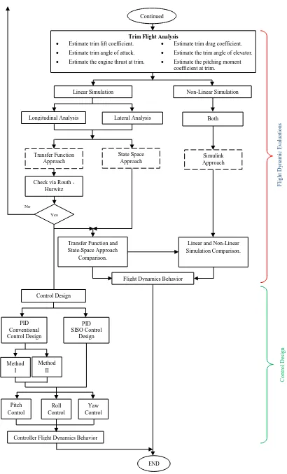
The present work focused on the development of computer code for the flight dynamic analysis and flight controller design of the fixed wing flying vehicle. Such work will involve three scope of works namely i) aerodynamic characteristic estimation, ii) the solution of flight dynamic equation of motion and iii) flight controller design. These three scopes of works are carried out sequentially as shown in the flow diagram as shown Figure 1.2 and can be explained as follows

(a) The first scope of aerodynamics characteristics will concern with the aerodynamic estimation by use a semi empirical aerodynamics estimation follows the method adopted from DATCOM [14], Ref [15] and Ref [16]. (b) The second scope concerned with deriving the governing equation of flight

motion in general form, trimmed flight, and their linearized form in longitudinal, lateral and directional flight direction. In this scope of work will involve in manner how to solve the trimmed flight equation, longitudinal flight equation, lateral and directional flight equation and the nonlinear flight equation by use of Simulink.

(c) The third scope related in the manner how to control flight behavior through the operation of the three control surfaces (elevator, aileron and rudder) and the engine thrust by use of PID controller scheme.

(d) The scope of work as stated in a, b and c will be converted into computer code written in MATLAB programming language.

(31)

7

Software Required Input Data

Mass and Moments of Inertia

 Aircraft mass.  Moment of inertia z-axis.

 Moment of inertia x-axis.  Moment of inertia xz-axis.

 Moment of inertia y-axis.

Estimates Primary Aerodynamic Characteristics CLo, Cmo, CLα,Cmα, CLq, Cmq, CLα, Cmα, Cyβ, Clβ, Cnβ , Cyp, ClP, Cnp,

Cyr, Clr, Cnr, CLδE, CmδE, CyδA , ClδA, CnδA, CyδR, CnδR, ClδR.

Perform believability

Coefficient Typically Coefficient Typically Coefficient Typically

Weight + Ixx + Izz +

Mass + Iyy + Ixz +

Ac of gravity 32.2 Wing span + Wing area +

Mean chord + CDmin 0.02 to 0.03 CDmin(point) 0.0

CLo 0.0 to 0.50 CLα 3.0 to 6.0 CLδ𝐸 0.3 to 0.9

CLα 1.0 to 8.0 CLq 4.0 to 10.0 Cyβ -0.3 to -1.0

CyδA <5.0 % of CyδR CyδR 0.1 to 0.2 Cyp 0.0 to - 0.3

Cyr 0 .2 to 0.5 Clβ - 0.09 to - 0.30 ClδA 0.05 to 0.2

ClδR 0.0 to 0.02 ClP - 0.30 to - 0.6 Clr 0.07 to 0.20

Cmo - 0.056358 Cmα - CmδE - 1.0 to – 2.0

Cmα – 3.0 to – 15.0 Cmq - 11 to – 30 Cnβ 0.06 to 0.2

CnδA <10 % of CnδR CnδR -0.06 to -0.12 Cnp -0.02 to -0.2

Cnr - 0.09 to -0.4

Yes

Start

Given Aircraft Configurations

 Wing Surface Area.  Mean Aerodynamic chord.

 Wing Span.  Other Geometric data.

Given Aircraft Flight Conditions

 Flight altitude.  True airspeed.

 Mach number.  Dynamic pressure.

 Location of CG in % MAC.  Steady-state angle of attack.

No

Dimensional Stability and Control Derivatives Xu, Xα, XTu, XδE, Mα,, Mu, MTα, MTu, Mα, Mq, MδE, Zu, Zα, Zα, Zq, ZδE,

Lβ, Lp, Lr, LδA, LδR, Nβ, NTβ, Np, Nr, NδA, NδR, Yβ, Yp, Yr, YδA, YδR.

(32)

[image:32.595.113.523.77.754.2]

8

Figure 1.2: Flight dynamics analysis and design procedure

C o n tr o l D esi g n

Controller Flight Dynamics Behavior Roll Control Yaw Control Pitch Control END Method I Method II Simulink Approach State Space Approach Transfer Function Approach

Check via Routh - Hurwitz

Non-Linear Simulation Linear Simulation

Continued

Longitudinal Analysis Lateral Analysis Both

Yes No

Transfer Function and State-Space Approach

Comparison.

Linear and Non-Linear Simulation Comparison.

Flight Dynamics Behavior

PID SISO Control Design Control Design PID Conventional Control Design F li g h t D y n ami c Ev al u at io n s

Trim Flight Analysis

 Estimate trim lift coefficient.  Estimate trim drag coefficient.

 Estimate trim angle of attack.  Estimate the trim angle of elevator.

(33)

9

1.5 Research methodology

In order to develop the capability in evaluating the flight dynamics in aircraft behavior and the ability to design a controllable flight behavior upon a particular flight variable, the proposed research methodology comprised of the following items: (i) Literature research.

(ii) Procurement and commissioning of language program software.

(iii) Collecting aircraft geometry data and estimating the aerodynamic characteristics needed in the equation of aircraft flight motion.

(iv) Solving the governing equation at trimmed flight condition.

(v) Solving the governing equation of flight motion in their linearized form. (vi) Solving the governing equation of flight motion in non-linear aircraft model

by using a Simulink

(vii) Controller design under longitudinal flight mode.

(viii) Controller design under lateral and directional flight modes.

The validation of each scope work in view of aerodynamics estimation are carried by comparing their result with the result provided by Ref [15] and [16], while in the relationship with the solution of equation of the flight motion are validated with the result provided by Ref [22]. In the control design with result adopted from Ref [23].

1.6 The results of the research work

The output of this research work had been in the form of software, which allows one to evaluate the flight dynamic behavior and the controlling flight behavior for a particular flight parameter. The software possessed the following capabilities:

(a) For a given aircraft configuration and flight condition, the software produced primary and derivatives aerodynamics characteristics.

(b) In addition to the given mass and the moment of inertia, the software produced the trimmed flight condition.

(34)

10

(d) Beginning with trim condition, the software evaluated all flight parameters that described the overall flight behavior by solving the non-linear governing equation of the flight motion.

(e) For a particular flight parameter, the software had been able to be used as a design tool for longitudinal or lateral–directional flight motion.

Considering the capabilities of the developed computer code as listed above, this software may very useful in the development of the Unmanned Aerial Vehicle (UAV) systems which currently had been attracted by almost all countries around the World to have them. This system can be developed from the Remotely Controller Aircraft (R.C Aircraft) in which such kind aircraft models are easily obtained in the market.

1.7 Organization of the thesis

This thesis is divided into five chapters. The first chapter describes the introduction chapter, including the problem statement, purpose objectives, scope of work, the research methodology, the results of the research work and the organization of the thesis.

(35)

11

software; the tenth section describes the flight dynamic software in gen eral and the section eleven provides the examples of flight dynamic software that had been developed in the past.

Chapter three of the present thesis describes how the flight equations of motions are solved and the manner of controlling the aircraft movement. Hence, this chapter includes the reviews on the research methodology that will be carried out, aerodynamic characteristics estimations, and also the manner of the dimensional stability and control derivatives to be determined. In addition to this, the solution of flight motion based on transfer function, state space formulation and the three PID controller design methods are discussed. Besides that, the non-linear aircraft simulations are also presented in this chapter.

The results and discussions are presented in chapter four. It starts from describing the aircrafts geometry, flight condition and mass and moments of inertia data of the aircraft under investigation. This chapter is divided into three sections. The first section is related to the longitudinal and lateral directional dynamic stability analysis with or without control surfaces in operation. Here, for the given aircraft data, one can evaluate how the flight variables such as aircraft speed u, angle of attack α, pitch angle θ, change with respect to time in corresponding to the longitudinal motion.

Flight variables are in terms of the side slip angle β, the Euler roll angle ϕ and the Euler yaw angle ψ with respect to time in relation with lateral motion. These various

(36)

CHAPTER 2

LITERATURE REVIEW

2.1 Aircraft flight dynamics

Flight dynamics is a branch of basic science of aeronautics that studies the flight behaviors of the aircraft during the flight in an atmosphere. This field, which is studied together with aerodynamics, aircraft structure and propulsion, plays an important role in the activities of designing a new aircraft [24]. The flight dynamics, as well as aerodynamics, represents a larger field of study. As a result, this field of study is normally split into 5 fields, as suggested by Hull [25]. They are i) trajectory analysis (performance), ii) stability and control, iii) aircraft sizing, iv) simulation and v) flight testing. Besides, Etkin [26] provides some examples of the main type of flight dynamics problems that occur in engineering practices, which are:

(a) Calculation of quantities performance, such as maximum flight speed, flight altitude, flight endurance, fuel consumption, takeoff, and landing distance. (b) Calculation trajectories, such as lunch, reentry, orbit, and landing.

(c) Stability of motion.

(d) Response of the vehicle due to control activation and due to propulsive change.

(37)

13

(f) Aero elastic oscillation (flutter).

(g) Assessment of human–pilot/machine combination (handling qualities).

Considering the types of problems mentioned above, the first two types of the problems can be categories as flight performance analysis. The scope of work involved in this analysis is quite a formidable task, as asserted by Ojha [27] that a performance analysis needs to be carried out for almost all phases of a flight, starting from takeoff, climb, cruise, turn, descent, and finally landing. In each phase of a flight, the aircraft may experience engine failure, so the aircraft flies at an unpowered flight or at a gliding flight condition. In addition to this, the performance analysis depends on the type of propulsive unit used with the specific types of aircraft.

(38)

14

overall, the aerospace industry, which includes military aircrafts and missiles, based on the results of market survey conducted by Boeing aircraft, manufacturer provides the revenue for aerospace industry from 2010 to 2020 at an amount of $ 3.60 trillion or yearly at around $ 180 billion [29]. Besides, the driving force in utilizing the flight dynamics knowledge may come from the development of aircraft for fulfilling the military purposes. Moreover, the ability to fly at a high angle of attack or at a higher speed and better maneuverability solve a lot of issues related to flight dynamics. In the past, building an aircraft with good stability characteristics that usually ensure good flying qualities can only be achieved with good aerodynamic design. Furthermore, in line with the development of automatic flight control systems (AFCS), provision of good flying qualities is no longer a guaranteed product in good aerodynamic design and good stability characteristics. This suggests that the study pertaining to flight dynamics should be presented in a new format; from conventional flight dynamics study to modern flight dynamics study. In this format, the modern flight dynamics is concerned not only with the dynamics, stability, and control of the basic airframe, but also with, sometimes, the complex interaction between airframe and flight control system. At present, the modern flight dynamists tend to be concerned with the wider issues of flying and handling qualities rather than with the traditional, as well as more limited issues of stability and control. As a result, the modern flight dynamics, as suggested by Cook[30], involves the work of:

(a) The establishment of a suitable mathematical framework for the problem, the development of the equations of motion, the solution of the equations of motion, investigation of response to controls, and the general interpretation of dynamic behavior.

(b) Reviewing on contemporary flying qualities requirements, as well as their evaluation and interpretation in the context of stability and control characteristics.

(c) The development of the feedback control if an aircraft has unacceptable flying qualities.

(39)

15

Hence, further difference among of them in imposing the assumptions, which of course will give a different form of governing equation of motion and how the governing equation of the corresponding equation should be solved, had been looked into. Thus, the governing equation of flight motion is presented in the following sub chapter and in sequence manner, followed by the simplification of the governing equation of flight motion, for the flight dynamics problem to be treatable.

2.2 The governing equation of flight motions

In flight, an aircraft can move in six degrees of freedom. The movement of the aircraft can take in three translational and three rotational movements. In order to understand the aircraft flight behavior, as well as to control the aircraft movement, one has to derive the governing equation of flight motion. This governing equation can reflect the possibility to determine the aircraft position, orientation, velocity, acceleration, forces, and moment acting on the flying vehicle. Unfortunately, all those quantities cannot be presented by just using a single coordinate system, as one needs to use more than coordinate systems. Moreover, specifying the position and the vehicle orientation requires one to define an inertial frame of coordinate system, while for the forces and the moments that act on the vehicle may be referred to the axis system attached to the flying vehicle. Strictly speaking, two coordinate systems need to be defined in formulating the governing equation of flight motion, and they are: i) the inertial coordinate reference system, and ii) the coordinate body fixed axis reference system. The inertial coordinate system is defined as a system coordinate, in which the Newton’s second law is applied[31].

In respect that the rotation of the Earth is relatively slow compared to the problems involving the dynamics of aircraft, the Earth can be selected as the inertial coordinate system of reference. Here, the selected coordinate system must be orthogonal and right-handed [32]. Basically, defining the inertial coordinate system on the Earth can be done in various manners; here, one can place the origin of the coordinate system at anywhere on the Earth. Let the coordinate system be denoted by the symbol (F) with a subscript intended to mnemonic the name of the corresponding coordinate system. If it is so, (FI) reflects the coordinate system of inertial frame. Meanwhile,

(40)

16

the system labeled as (x, y, and z) and the companion with an appropriate subscript (I), they become (xI, yI, and zI). The unit vectors, along with x, y, and z, are denoted

as (i, j, and k) respectively. Besides, with the earth being selected as the place of an inertial coordinate system, it had been identified that three models of the inertial coordinate system are commonly used in solving the flight dynamic problems, which are:

(a) The Earth-centered reference frame, (FEC), as shown in Figure 2.1a.

(b) The Earth-fixed reference frame, (FE), as shown in Figure 2.1b.

(c) The local-horizontal reference frame, (FH), as shown in Figure 2.1c.

(a) (b)

[image:40.595.115.525.271.736.2]

(c)

(41)

17

Figures 2.1a, b, and c illustrate the placements of their origin of the coordinate systems for the above three types of inertial coordinate systems.

If one chooses one of those three reference frames as its inertial coordinate axis system, one has to be consistently used in the whole process of solving the flight dynamics problems. However, it had been identified that most of the flying vehicles in the atmospheres, as far as the flight speed below the hypersonic speed, a local horizontal reference frame is preferred [34].

Meanwhile, the second coordinate system, besides the inertial coordinate system, is a body fixed axis reference system. This coordinate system, assigned to have the origin and the axes of the coordinate system, is fixed with respect to the geometry of the aircraft. Here, three types of body fixed coordinate systems can be applied, and they are:

(a) Body axis fixed coordinate systems. (b) Stability axis fixed coordinate systems. (c) Wind axis fixed coordinate systems.

These three coordinate systems are used in the aircraft’s center of gravity (C.G) as its origin, and in defining the y and the z axes, they share the same orientation. Their difference occurs in terms of defining the orientation of the x-axis, as depicted in Figure 2.2. The x-axis of body axis fixed coordinate system normally coincides or is parallel to the axis of fuselage. Meanwhile, the x-axis of stability axis fixed coordinate is parallel with a line drawn to indicate that the present aptitude of aircraft makes an angle of attack α to the incoming air velocity, whereas the x-axis of wind

(42)

[image:42.595.129.506.74.280.2]

18

Figure 2.2: The orientation of body axis, stability axis, and wind axis [34]

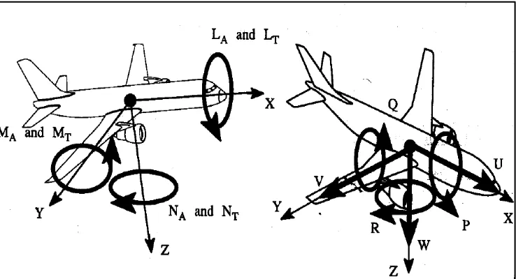
In respect to the inertial frame of reference, the orientation of body axis coordinate system is shown in Figure 2.3. In addition, forces and moments, as well as the definitions of linear and angular velocities on the body axis are shown in Figure 2.4.

[image:42.595.133.506.413.614.2]

(43)

19

[image:43.595.120.519.67.293.2]

(a) (b)

Figure 2.4a: Definitions of aerodynamic forces, thrust and acceleration gravitation in body axis coordinate system [34]

Figure 2.4b: Definitions of moments, linear, and angular velocity in body axis coordinate system [33]

[image:43.595.135.504.361.561.2]

(44)

[image:44.595.115.526.109.250.2]

20

Table 2.1: The definitions of notations in describing forces, moment, and velocity components [34]

NO DEFINITION ROLL AXIS xb PITCH AXIS yb YAW AXIS zb

1 Angular rate p q r

2 Velocity components u v w

3 Aerodynamic force components X Y Z

4 Aerodynamics moment components L M N

5 Moment of inertia about each axis Ixx Iyy Izz

6 Product of inertia Iyz Ixz Ixy

7 Engine thrust T ….. …..

Basically, the governing equation of flight motion can be broken down into two groups [31]. The first group is the governing equation of flight motion derived from the implementation of the Newton’s second law to the aircraft. Meanwhile, the

second group of equations is developed based on the kinematic relationship between the inertial axis reference systems and the body fixed reference system [35].

As mentioned previously, the inertial coordinate system is employed to specify the aircraft position, orientation, velocity, and the aircraft acceleration. In other words, this inertial coordinate system allows one to apply the Newton’s second law to the aircraft. If the aircraft mass is denoted as (m); the aircraft with respect to the inertial

reference system moves in varying directions based on the vector velocity ⃗⃗ , and

the forces acting on the aircraft ( ⃗ ), hence, the Newton’s second law states that for

the given force ( ⃗ ), there is equal time rate of change in its linear momentum ̅ .

Meanwhile, if ⃗⃗⃗ represents the external moment applied on the aircraft, the moment ⃗⃗⃗ will be equal to the time rate of angular momentum ⃗⃗ . These two statements can be written mathematically as:

⃗ ⃗⃗ (2.1a)

⃗⃗⃗ ⃗⃗ (2.1b)

(45)

21

hence the term

⃗⃗ |can be written in terms of ⃗⃗ | by using the

following relation:

⃗⃗ | ⃗⃗ | ⃗⃗ | ⃗⃗ | (2.2a)

In a similar manner, the rate change of angular momentum, which was previously written with respect to inertial coordinate system, then completely can be written with respect to the body fixed coordinate in the following relation.

⃗⃗ | ⃗⃗ | ⃗⃗ | ⃗⃗ | (2.2b)

Equation 2.2 is substituted to Equation 2.1; which gives the representation of the Newton’s second law in body fixed reference frame as:

⃗ | ⃗⃗ |

⃗⃗ | ⃗⃗ | (2.3a)

⃗⃗⃗ | ⃗⃗ |

⃗⃗ | ⃗⃗ | (2.3b)

If the vector unit of the body axis system (xyz) for x-axis is denoted by , y-axis is

denoted by , and z-axis is denoted with its unit vector ⃗ , and hence, the two

vectors, velocity ( ⃗⃗ and angular velocity ( ⃗⃗ , can be equated as:

⃗ ⃗ (2.4a)

⃗⃗ ⃗ (2.4b)

The externally applied aerodynamic forces ⃗ , and moments ⃗⃗⃗ that act on the aircraft are primarily due to airflow condition and their control surface deflections. In

a similar manner with vector velocity ⃗⃗ and vector angular velocity ⃗⃗ , this

applied force ⃗ and moment ⃗⃗⃗ , as well as angular momentum (⃗⃗ , can be broken down into vector components along the longitudinal (x), the lateral (y), and the vertical axis (z) of the body fixed reference frame. Besides, the force components in the longitudinal, lateral, and vertical axes are denoted as (Fx), (Fy), and (Fz)

respectively. During application, the moment ⃗⃗⃗ is denoted in terms of its component as (L), (M), and (N). On the other hand, the vector angular momentum ⃗⃗ associated with their components in body fixed reference is denoted as (Hx),

(Hy), and (Hz). Hence, the forces and the moments, as stated in Equations 2.1a and

2.1b, are written in the form of scalar notation as:

(46)

22

(2.5b)

(2.5c)

(2.6a)

(2.6b)

(2.6c)

The vector angular momentum ⃗⃗ , in conjunction with the vector angular velocity ⃗⃗ , can be written as:

⃗⃗ [

] ⃗⃗ (2.7)

In assuming that the aircraft mass (m) is a constant and by substituting Equation 2.7 into Equations 2.5 and 2.4, one can write these two equations in scalar form as:

̇ (2.8a)

̇ (2.8b)

̇ (2.8c)

̇ ̇ ̇ ( )

(2.9a)

̇ ̇ ̇

(2.9b)

̇ ̇ ̇ ( )

(2.9c) The left hand side of the above equations represents the external forces and moments. These forces and moments are due to aerodynamic forces, aircraft weight, and engine thrust, which can be written in the following forms:

̅ (2.10a)

̅ (2.10b)

̅ (2.10c)

As for the moments, they can be written as in the following:

̅ (2.11a)

̅ (2.11b)

(47)

23

The definitions of notations that appear in the right hand side of Equations 2.10 and 2.11 are given in the list of symbols.

In other forms, the force equations (Equation 2.10) can be written as:

̇ ̅ (2.12a)

̇ ̅ (2.12b)

̇ ̅ (2.12c)

Meanwhile, the momentum Equations (Equation 2.11) can be written as:

̇ ̇ ̇ ̅ ( ) (2.13a) ̇ ̇ ̇ ̅ (2.13b) ̇ ̇ ̇ ̅ ( ) (2.13c)

Furthermore, in a relationship between a body axis fixed coordinate system and the Earth-fixed reference frame, the rotational velocity with respect to the body axis fixed coordinate system is described by the variables (r, p, and q), while the Earth

fixed coordinate system is described by ( ̇, ̇, and ̇). The relationship between these two triples is shown in [31]:

[ ] [ ] [ ̇ ̇ ̇

] (2.14)

The above relationship indicates that if the body axis fixed coordinate system is placed parallel to the Earth fixed coordinate system, which means (θ = 0.0 and ϕ =

0.0), one will obtain ( ̇, ̇ and ̇). Hence, they show the angular rate of the vehicle to the inertial frame of reference. Besides, the above equation (Equation 2.14) can be solved to represent how the aptitude of the flying vehicle changes with the inertial frame of reference by inversing that equation and provides the result as:

[ ̇ ̇ ̇ ] [

] [ ] (2.15)

(48)

24

[

]

[

] [ ] (2.16)

Equation 2.12 to Equation 2.16 represents the governing equation of aircraft flight motion. These equations contain 12 state variables, which are sufficient in describing the flight behavior of the aircraft.

In addition to these 12 state variables, one may add three other state variables: i) the total velocity (V), ii) the angle of attack α, and iii) the side slip angle β. These three

state variables can be derived from the component velocities (u, v, and w) as depicted in the following:

√ (2.17a)

( ) (2.17b)

( ) (2.17c)

If one applies the first derivative with respect to time into these three above equations, one can obtain:

̇ ̇ ̇ ̇ (2.18a)

̇ ̇ ̇ (2.18b)

̇ ( ) ̇ ̇ ̇

√ (2.18c)

If ̇, ̇ and ̇ , which are defined by Equation 2.12, are substituted into the above equations, the results are:

̇ (2.19a)

̇ (2.19b)

̇ (2.19c)

With the definitions of (Fx, Fy, and Fz), as given by Equation 2.10 into Equation 2.19,

one obtains the state variables (V, α and β) as: ̇

̅

(49)

221

REFERENCES

1. Jenie, Said D., and Agus Budiyono. "Automatic Flight Control System-Classical approach and modern control perspective." Indonesia: Department

of Aeronautics and Astronautics-ITB 2006.

2. Pratt, Roger. Flight control systems: practical issues in design and

implementation. No. 57. Iet, 2000.

3. Kuo, Benjamin C. Automatic control systems. Prentice Hall PTR, 1981. 4. Pearsall, Jr Earle S. and Richolt Robert. "Aircraft control system." U.S. Patent

No. 2,389,274. 20 Nov. 1945.

5. Collinson, R. P. G. "Fly-by-wire flight control." Introduction to Avionics

Systems. Springer Netherlands, 2011. 179-253.

6. McLean, Donald. "Automatic flight control systems (Book)." Englewood

Cliffs, NJ, Prentice Hall, 1990, 606 (1990).

7. Franklin, Gene F., J. David Powell, & Abbas Emami-Naeini. "Feedback

Control of Dynamics Systems." Prentice Hall Inc. 2006.

8. McRuer, Duane T., Dunstan Graham, and Irving Ashkenas. Aircraft dynamics

and automatic control. Princeton University Press, 2014.

9. Cook, Michael V. Flight dynamics principles: a linear systems approach to

aircraft stability and control. Butterworth-Heinemann, 2012.

10. Babister, Arthur William. Aircraft Dynamic Stability and Response: Pergamon International Library of Science, Technology, Engineering and

Social Studies. Elsevier, 2013.

11. Blakelock, John H. Automatic control of aircraft and missiles. John Wiley & Sons, 1991.

(50)

222

13. Stevens, Brian L., and Frank L. Lewis. Aircraft control and simulation. John Wiley & Sons, 2003.

14. Blake, William B. Missile Datcom: User's Manual-1997 FORTRAN 90

Revision. No. AFRL-VA-WP-TR-1998-3009. AIR FORCE RESEARCH

LAB WRIGHT-PATTERSON AFB OH AIR VEHICLES DIRECTORATE, 1998.

15. Roskam, Jan. Airplane Design: Part 2-Preliminary Configuration Design and

Integration of the Propulsion System. DARcorporation, 1985

16. Roskam, Jan. "Airplane Design: Part I-VIII." DARcorporation, Lawrence, KS

2006

17. Steuernagle, J., K. Roy, and S. Ells. "Cessna 182 Skylane Safety Highlights."AOPA Air Safety Foundation, Marylan, 2001.

18. DAVID, FRED R., and NANCY MARLOW. "CESSNA AIRCRAFT CORPORATION." Journal of management case studies 1986: 33.

19. Plans, Model Airplane, et al. "The current top posts." Archives of top posts. 2013.

20. Goritschnig, Guenther, et al. "The Evolution of Civil Aircraft Design at Bombardier: An Historical Perspective." CASI Conference Proceedings. 2003.

21. Field, H. "EUROPE'S AIR TAXIS." Flight International 115.3647 1979. 22. Marcello Napolitano, Aircraft dynamics: From modeling to Simulation, 2012. 23. Lie, Karen. "Cruise Control System in Vehicle." Michigan: Calvin College.

1982

24. Stengel, Robert F. Flight dynamics. Princeton University Press, 2015. 25. Hull, David G. "Fundamentals of Airplane Flight Mechanics." 2007.

26. Etkin, Bernard. "Dynamics of Atmospheric Flight, John Wiley and Sons." Inc, New York, London, Sydney 1972.

27. Ojha, S.K.: Flight Performance of Aircraft, AIAA, Inc. Washington, DC, USA, 1995.

28. Benkard, C. Lanier. "A dynamic analysis of the market for wide-bodied commercial aircraft." The Review of Economic Studies 71.3 2004: 581-611. 29. Airplanes, Boeing Commercial. "Current Market Outlook:

(51)

223

30. Cook, Michael V. Flight dynamics principles: a linear systems approach to

aircraft stability and control. Butterworth-Heinemann, 2012.

31. Nelson, Robert C. Flight stability and automatic control. Vol. 2. WCB/McGraw Hill, 1998.

32. Pamadi, Bandu N. Performance, stability, dynamics, and control of airplanes. Aiaa, 2004.

33. Durham, Wayne. Aircraft Flight Dynamics and Control. John Wiley & Sons, 2013.

34. Roskam, Jan. Airplane Flight Dynamics and Automatic Flight Controls. DAR Corporation, 1995.

35. Etkin, Bernard. Dynamics of atmospheric flight. Courier Corporation, 2012. 36. Maine, Richard E., and Kenneth W. Iliff. "Application of parameter

estimation to aircraft stability and control." NASA RP-1168 .1986.

37. Bryan, George Hartley. Stability in aviation: an introduction to dynamical

stability as applied to the motions of aeroplanes. Macmillan and Co., limited,

1911.

38. Roskam, Jan, and William A. Anemaat. General aviation aircraft design

methodology in a PC environment. No. 965520. SAE Technical Paper, 1996.

39. Russell, J. Performance and stability of aircraft. Butterworth-Heinemann, 1996.

40. Pamadi, Bandu N. Performance, stability, dynamics, and control of airplanes. Aiaa, 2004.

41. McLean, Marie. California Women: Activities Guide, Kindergarten through

Grade Twelve. Publications Sales, California State Department of Education,

PO Box 271, Sacramento, CA 95802-0271, 1988.

42. Faghihi, F., and K. Hadad. "Numerical solutions of coupled differential equations and initial values using Maple software." Applied Mathematics and Computation 155.2 (2004): 563-572.

43. Chandrasekaran, S., and A. K. Jain. "Dynamic behaviour of square and triangular offshore tension leg platforms under regular wave loads." Ocean

Engineering 29.3, 2002: 279-313.

(52)

224

45. Garza, Frederico R., and Eugene A. Morelli. "A collection of nonlinear aircraft simulations in matlab." NASA Langley Research Center, Technical

Report NASA/TM 212145, 2003.

46. Etkin, Bernard, and Lloyd Duff Reid. Dynamics of Flight: Stability and Control. Vol. 3. New York: Wiley, 1996.

47. Dustman, Larry L. "Transmitter extension apparatus for manipulating model vehicles." U.S. Patent No. 4,386,914. 7 Jun. 1983.

48. Wassily W. Leontief, Faye Duchin (2004). World Wide Military Last Update: January 6th, 2008: from: http://www.worldwide-military.com

49. Fischel, Eduard. "Aileron control for airplanes." U.S. Patent No. 2,137,974. 22 Nov. 1938.

50. Plan, NASA Strategic. "National Aeronautics and Space Administration."Washington, DC, February , 1995.

51. "Aircraft elevator construction." U.S. Patent 2,430,793, issued November 11, 1947.

52. Fahey, James Charles. The Ships and Aircraft of the US Fleet. Naval Institute Press, 1958.

53. Carl, Udo. "Drive control for a vertical rudder of an aircraft." U.S. Patent No. 4,759,515. 26 Jul. 1988.

54. Lin, Ching-Fang. "Aircraft rudder command system." U.S. Patent No. 5,170,969. 15 Dec. 1992.

55. Burcham, Frank W., and Charles Gordon Fullerton. Controlling Crippled

Aircraft--with Throttles. National Aeronautics and Space Administration,

Ames Research Center, Dryden Flight Research Facility, 1991.

56. Robbins, Richard E., and Robert D. Simpson. "Method and apparatus for aircraft pitch and thrust axes control." U.S. Patent No. 4,471,439. 11 Sep. 1984.

57. Miller, Robert A. "Current status of thermal barrier coatings—an overview."Surface and Coatings Technology 30.1 1987: 1-11.

58. Burcham, Frank W., et al. "Engines-only flight control system." U.S. Patent No. 5,330,131. 19 Jul. 1994.

(53)

225

60. Young, Harvey R. "Power management system." U.S. Patent No. 4,488,851. 18 Dec. 1984.

61. Ang, Kiam Heong, Gregory Chong, and Yun Li. "PID Control System Analysis, Design, and Technology." Control Systems Technology, IEEE Transactions on13.4, 2005: 559-576.

62. Åström, Karl Johan, and Tore Hägglund. Advanced PID control. ISA-The Instrumentation, Systems, and Automation Society; Research Triangle Park, NC 27709, 2006.

63. Kiong, Tan Kok, et al. "Modern Designs." Advances in PID Control. Springer London, 1999. 35-97.

64. Smetana, Frederick O., Delbert Clyde Summey, and W. Donald Johnson.Riding and Handling Qualities of Light Aircraft: A Review and

Analysis. National Aeronautics and Space Administration, 1972.

65. Smetana, F. O., "Aircraft Performance, Stability and Control," Aircraft Designs, Inc., Monterey, CA, 1988.

66. Smetana, F. O., "Aircraft Performance, Stability and Control," Aircraft Designs, Inc., Monterey, CA, 2000.

67. Smetana, F. O., Summey, D. C., and Johnson, W. D., "Point and Path

Performance of Light Aircraft—A Review and Analysis," NASA CR 2272,

June 1973.

68. Fink, R. D., and D. E. Hoak. "USAF stability and control DATCOM." Air

Force Flight Dynamics Laboratory, Wright-Patterson AFB, Ohio ,1975.

69. Williams, John E., and Steven R. Vukelich. The USAF stability and control

digital dATCOM. Volume I. Users manual. MCDONNELL DOUGLAS

ASTRONAUTICS CO ST LOUIS MO, 1979.

70. Jelinski, Z., and P. B. Moranda. "Software reliability research, Statistical Computer Performance Evaluation, W. Freiberger (ed.), 465–484." 1972. 71. Sukert, Alan N. "Empirical validation of three software error prediction

models."Reliability, IEEE Transactions on 28.3 (1979): 199-205.

72. Maskew, Brian. "Program VSAERO theory document." NASA CR-4023 , 1987.