Results in Sizing and Simulation of PV Applications Based on Different Solar Cell Technologies

http://www.scirp.org/journal/jpee ISSN Online: 2327-5901

ISSN Print: 2327-588X

Results in Sizing and Simulation of PV

Applications Based on Different Solar Cell

Technologies

Alexandru Diaconu

, Laurentiu Fara

, Paul Sterian

, Dan Craciunescu

, Silvian Fara

1_{University Politehnica, Bucharest, Romania}

2_{Academy of Romanian Scientists, Bucharest, Romania}

Abstract

Modeling and simulation of photovoltaic (PV) systems represents an essential task for the integration of PV panels in current power applications. At the present time, there are sizing tools of photovoltaic systems available on the market, taking into account the proposed energy consumption, site localiza-tion and system cost. An advanced specialized program (PVSyst) was consi-dered. The sizing and simulations of two PV important applications were de-veloped using PV modules based on three different technologies: monocrys-talline and polycrysmonocrys-talline silicon, as well as CIS. Our results showed how dif-ferent types of solar cell technologies influenced the final power output and performances for a PV LED lighting, as well as for a PV water pumping sys-tem, in terms of overall yield, efficiency and system availability.

Keywords

Photovoltaic, Simulations, Monocrystalline, Polycrystalline, Copper Indium Selenide, Solar Cells, Photovoltaic Lighting, Photovoltaic Water Pumping System

1. Introduction

Photovoltaic systems have a wide range of applicability and also include public or privately owned solar-powered lighting systems or solar powered water pumps

[1]. Solar pumps offer a clean and simple alternative to fuel-burning engines and generators for domestic water, livestock and irrigation [2]. They are most effec-tive during dry and sunny seasons. They require no fuel deliveries, and very little maintenance. Solar-powered lighting is an effective way to implement illumina-tion soluillumina-tions in terms of technology and consumpillumina-tion [3]. Global pressures How to cite this paper: Diaconu, A., Fara,

L., Sterian, P., Craciunescu, D. and Fara, S. (2017) Results in Sizing and Simulation of PV Applications Based on Different Solar Cell Technologies. Journal of Power and Energy Engineering, 5, 63-74.

http://dx.doi.org/10.4236/jpee.2017.51005

Received: December 13, 2016 Accepted: January 16, 2017 Published: January 19, 2017

Copyright © 2017 by authors and Scientific Research Publishing Inc. This work is licensed under the Creative Commons Attribution International License (CC BY 4.0).

were made to protect the environment, which has become a priority. In meeting these types of problems, various systems have been developed to replace tradi-tional lighting with energy efficient lighting. The most common method is the LED (Light Emitting Diode) technology.

Various system simulations and dimensioning were developed for specific re-gions and applications, but using only one type of PV technology. In the paper “Performance analysis of a 190 kWp grid interactive solar photovoltaic power plant in India”, V. Sharma and S. S. Chandel have used polycrystalline modules to assess the performance of a power plant installed in India [4].

In the paper called “Simulation and performance analysis of 110 kWp grid- connected photovoltaic system for residential building in India: A comparative analysis of various PV technology”, a similar approach is considered for a system to be implemented in a residential building in India. Four types of PV technolo-gies were simulated to determine performance ratios and energy yield [5].

The purpose of the present paper is to identify the best solar cell technology that offers the highest system performances in a specific location. In order to de-fine the most efficient solution that could be implemented in a given location, simulations were developed using monocrystalline, polycrystalline and CIS pho-tovoltaic modules [6].

2. Real-Life Usage

Solar-powered lighting is an effective way to implement illumination solutions in terms of technology and consumption. Global pressures were made to protect the environment, which has become a priority. In meeting these types of prob-lems, various systems have been developed to replace traditional lighting with energy efficient lighting. The most common method is the LED technology (Light Emitting Diode).

The design and simulation also provides general information and guidelines on planning and designing of small solar powered water pump system for use in irrigation and livestock feeding operations. One benefit of using solar energy to power water pump systems is that increased water requirements tend to coincide with the seasonal increase of incoming solar energy. When properly designed, these systems can also result in significant long-term cost savings. Aside irriga-tion and livestock feeding operairriga-tions, these systems can and are being used for potable water supply in underdeveloped countries. As more and more ground-water sources become unsafe for drinking purposes, potable ground-water often needs to be drawn from depths that require pumping. A Solar-Powered Water Pumping System uses solar energy to power a pump to supply a village with potable water. Solar pumping systems are also commonly being used where it is too far to walk to a well or where the well only provides seasonally usable water.

3. About PVSyst Simulation Software

manages various types of photovoltaic system analysis like stand-alone PV sys-tems, grid connected of hybrid systems. PVSyst uses meteorological data from international databases as well as detailed information about the component tech-nical specifications [7].

4. Sizing and Simulations for PV LED Lighting System

We have chosen the PVSyst software application for comparing various solar cell technologies that could power a photovoltaic lighting system. In order to obtain conclusive results, we varied only the solar cell technologies, but the other com-ponents of the system remained unchanged. The sizing for this type of system will be as a stand-alone type, meaning that connection to the local energy grid is not required. Most of this type of systems require means for energy storage, therefore our system will use a solar battery. The PV application must be dimen-sioned to fully charge the batteries when exposed to maximum intensity for the given application. To avoid the possibility of damaging the system because of solar radiation fluctuations or battery overload, the system will be equipped with a charge controller.

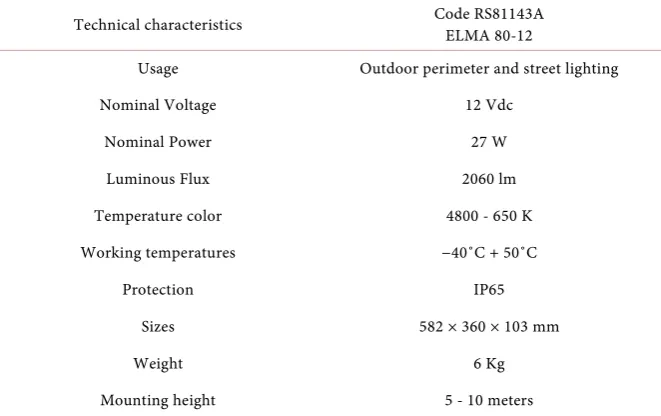
One of the main components of the system is the lighting fixture (Figure 1). This is an ELMA 80-12 component provided by Electromagnetica SA, a compa-ny that specialized in manufacturing LED system components for lighting fix-tures, and provides the following advantages: easy configuration and install, ecologic product, very high energy efficiency, low heat emissions, high reliability coefficient, low maintenance costs. The main technical parameters provided by Electromagnetica SA in the product technical sheet for the lighting fixture are presented in Table 1, as follows [8].

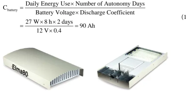
The PV system is intended to provide two days autonomy, in order to com-pensate for days with high cloudiness. This feature will result in a slightly over-sized PV generator and battery. The types of PV technologies used in the simu-lations are monocrystalline silicon, polycrystalline silicon and CIS solar cells. In order to choose the most suited solar battery for the system, important factors are considered, like daily energy consumption (27 W), number of days for sys-tem autonomy (2 days), battery voltage (12 V) and discharge coefficient (0.4). To obtain the battery capacity, the following equation was used [9]:

battery

Daily Energy Use Number of Autonomy Days C

Battery Voltage Discharge Coefficient

27 W 8 h 2 days

90 Ah 12 V 0.4

× =

× × ×

= =

×

(1)

Table 1. Main technical characteristics of ELMA LED.

Technical characteristics Code RS81143A _{ELMA 80-12}

Usage Outdoor perimeter and street lighting

Nominal Voltage 12 Vdc

Nominal Power 27 W

Luminous Flux 2060 lm

Temperature color 4800 - 650 K

Working temperatures −40˚C + 50˚C

Protection IP65

Sizes 582 × 360 × 103 mm

Weight 6 Kg

Mounting height 5 - 10 meters

Taking this result in consideration, for all the different types of PV technolo-gies used in the simulations, we have considered a Deka battery of 12 V/90 Ah. The solar radiation data for the photovoltaic generators were required from Me-teonorm database for Bucharest site and is presented in Table 2[10], as monthly daily values [kWh/m2_/day].

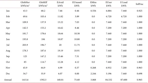
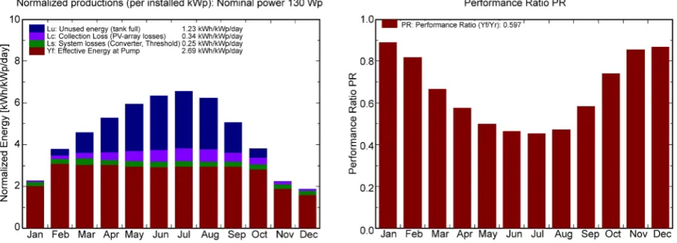
Table 3 represents the numerical simulation results for the LED system using monocrystalline silicon modules, while Figure 2 shows the normalized energy and the performance ratio of the system.

The simulation results of the photovoltaic system using monocrystalline sili-con shows that for January, November and December months, the system fails to provide 3068 kWh of energy needed. A quantity of 75.68 kWh is lost due to the battery capacity. This problem could be adjusted by lowering the power of the PV modules.

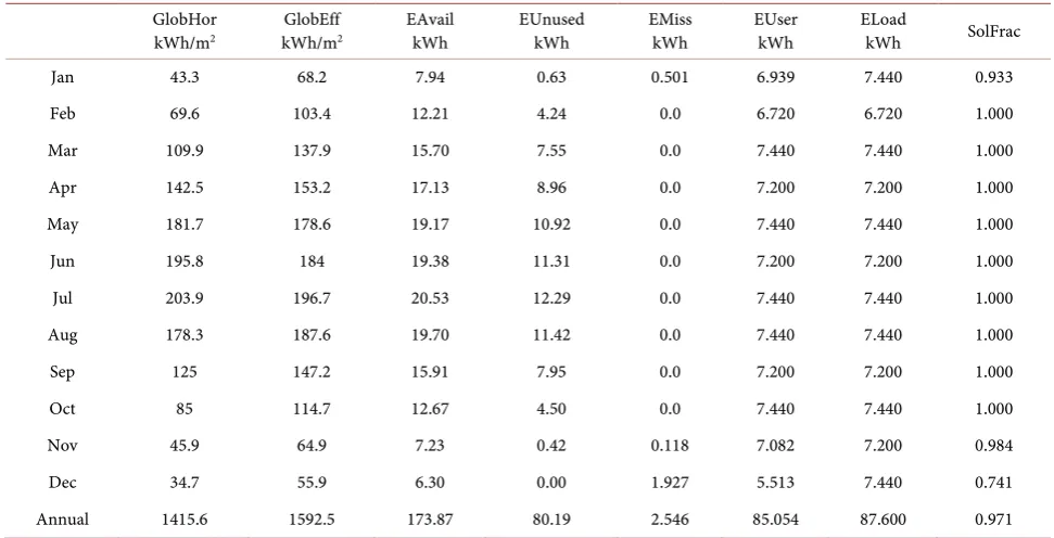
In Table 4, the numerical simulation results for the LED PV system using po-lycrystalline silicon are presented, while Figure 3 shows the normalized energy and the performance ratio of the PV system.

Results using polycrystalline silicon, as well as the monocrystalline silicon in-dicate that in January, November and December, the system cannot fulfill the total system energy needs, by a quantity of 2546 kWh. Battery losses are also present in the quantity of 80.19 kWh. This could also be adjusted by using smaller PV modules but, it is important to take into consideration the solar re-sources in the months that with low solar radiation.

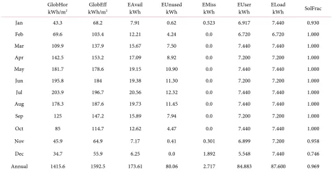
In Table 5, numerical simulation results for the PV LED system using CIS (Copper, Indium and Selenium) cells are presented, while Figure 4 shows the normalized energy and the performance ratio of the system.

Table 2. Mean daily values for Bucharest location.

Jan Feb Mar Apr May Jun Jul Aug Sep Oct Nov Dec

Hor. Global 1.40 2.49 3.55 4.75 5.86 6.53 6.58 5.75 4.17 2.74 1.53 1.12

Hor. diffuse 0.76 1.04 1.50 2.32 2.49 2.64 2.67 2.37 1.84 1.24 0.96 0.65

Clrn. index 0.39 0.48 0.5 0.51 0.53 0.56 0.58 0.57 0.52 0.47 0.38 0.36

Amb. Temp. −1 1.5 6.7 11.8 17.9 21.1 23.7 23.4 17.1 11.9 6.4 0.4

Table 3. Monthly numerical simulation results for PV LED system using monocrystalline silicon modules.

GlobHor

kWh/m2 _kWh/mGlobEff 2 EAvail _kWh EUnused _kWh EMiss _kWh EUser _kWh E Load _kWh SolFrac

Jan 43.3 68.2 7.66 0.46 0.556 6.884 7.440 0.925

Feb 69.6 103.4 11.82 3.89 0.0 6.720 6.720 1.000

Mar 109.9 137.9 15.22 7.03 0.0 7.440 7.440 1.000

Apr 142.5 153.2 16.62 8.46 0.0 7.200 7.200 1.000

May 181.7 178.6 18.64 10.38 0.0 7.440 7.440 1.000

Jun 195.8 184 18.87 10.80 0.0 7.200 7.200 1.000

Jul 203.9 196.7 20 11.75 0.0 7.440 7.440 1.000

Aug 178.3 187.6 19.19 10.91 0.0 7.440 7.440 1.000

Sep 125 147.2 15.46 7.51 0.0 7.200 7.200 1.000

Oct 85 114.7 12.28 4.12 0.0 7.440 7.440 1.000

Nov 45.9 64.9 6.99 0.37 0.268 6.932 7.200 0.963

Dec 34.7 55.9 6.07 0.00 2.244 5.196 7.440 0.698

Annual 1415.6 1592.5 168.81 75.68 3.068 84.532 87.600 0.965

where: -GlobHor represents Horizontal global irradiation; -GlobEff represents Effective global irradiation corrected for IAM and shadings, where IAM is the Incidence Angle Modifier; -EAvail represents the produced solar energy; -EUnused represents losses due to unused energy; -EMiss represents the missing energy in order for the system to function; -EUser represents the energy supplied to the user; -ELoad represents the energy needed of the user; -SolFrac represents the Solar Fraction, which is calculated as EUser/ELoad [11].

Table 4. Monthly numerical simulation results for PV LED system using polycrystalline silicon modules. GlobHor

kWh/m2 _kWh/mGlobEff 2 EAvail _kWh EUnused _kWh EMiss _kWh EUser _kWh ELoad _kWh SolFrac

Jan 43.3 68.2 7.94 0.63 0.501 6.939 7.440 0.933

Feb 69.6 103.4 12.21 4.24 0.0 6.720 6.720 1.000

Mar 109.9 137.9 15.70 7.55 0.0 7.440 7.440 1.000

Apr 142.5 153.2 17.13 8.96 0.0 7.200 7.200 1.000

May 181.7 178.6 19.17 10.92 0.0 7.440 7.440 1.000

Jun 195.8 184 19.38 11.31 0.0 7.200 7.200 1.000

Jul 203.9 196.7 20.53 12.29 0.0 7.440 7.440 1.000

Aug 178.3 187.6 19.70 11.42 0.0 7.440 7.440 1.000

Sep 125 147.2 15.91 7.95 0.0 7.200 7.200 1.000

Oct 85 114.7 12.67 4.50 0.0 7.440 7.440 1.000

Nov 45.9 64.9 7.23 0.42 0.118 7.082 7.200 0.984

Dec 34.7 55.9 6.30 0.00 1.927 5.513 7.440 0.741

Annual 1415.6 1592.5 173.87 80.19 2.546 85.054 87.600 0.971

Figure 3. Normalized energy productions, system performance ratio and solar fraction for PV LED system using polycrystalline

silicon modules.

Table 5. Monthly numerical simulation results for PV LED system using modules with CIS cells. GlobHor

kWh/m2 _kWh/mGlobEff 2 EAvail _kWh EUnused _kWh EMiss _kWh EUser _kWh ELoad _kWh SolFrac

Jan 43.3 68.2 7.91 0.62 0.523 6.917 7.440 0.930

Feb 69.6 103.4 12.21 4.24 0.0 6.720 6.720 1.000

Mar 109.9 137.9 15.67 7.50 0.0 7.440 7.440 1.000

Apr 142.5 153.2 17.09 8.92 0.0 7.200 7.200 1.000

May 181.7 178.6 19.15 10.90 0.0 7.440 7.440 1.000

Jun 195.8 184 19.38 11.30 0.0 7.200 7.200 1.000

Jul 203.9 196.7 20.56 12.32 0.0 7.440 7.440 1.000

Aug 178.3 187.6 19.73 11.45 0.0 7.440 7.440 1.000

Sep 125 147.2 15.89 7.94 0.0 7.200 7.200 1.000

Oct 85 114.7 12.62 4.47 0.0 7.440 7.440 1.000

Nov 45.9 64.9 7.17 0.41 0.301 6.899 7.200 0.958

Dec 34.7 55.9 6.25 0.0 1.892 5.548 7.440 0.746

Annual 1415.6 1592.5 173.61 80.06 2.717 84.883 87.600 0.969

Figure 4. Normalized energy productions, system performance ratio and solar fraction for PV LED system using modules with

CIS solar cells.

5. Sizing and Simulations for PV Water Pumping System

The PV pumping systems are able to deliver water both for irrigation and local water supply. These pumps are usually using direct current for operation that means that the power could be delivered straight from the PV modules. The pumps that use alternative current are also used but have some disadvantages, for example the system components are more complex and the yield drops when the type of current is changed by inverter.

In order to simulate a PV pumping system properly, we have used specific steps for choosing the right components of the system [12]. These steps are:

2-identification of the water supply,

3-identification all necessary components and their location, 4-designing a water storage component,

5-solar availability,

6-identification of needed water flow, 7-identification of total dynamic head pump, 8-pump selection and nominal power, 9-PV system design.

The project simulates the need of water in a farm in Romania. The water need for the project is calculated for 100 cattle. The farm area is contained in 16 hec-tares of land. We need that the system will be able to supply water in the period of May-September from a water well, when the animals are grazing. A storage tank will also be used, to store the water in order for the system to function in periods with clouds or poor solar availability [13]. A comparison between the different types of PV cells is made and the results are presented in the following tables and figures.

Figure 5 represents the simulation of the PV water pumping system using polycrystalline cell technology.

Table 6 represents the numerical simulation results for polycrystalline cell technology on an average monthly basis.

The results show that from the annual needed water amount of 1460 m3_{, the} system provided an amount of 1331 m3_{. Energy in the amount of 46 kWh was} lost due to the system oversize and annual, the amount of 8.9 % of water was not provided. Months in which the system is unable to provide water are January, February and December. This is due to the low solar radiation availability needed to power the system.

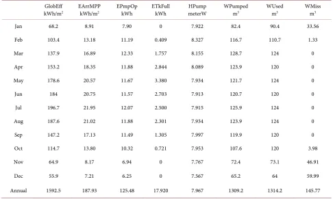
Table 7 represents the numerical simulation results for the PV pumping sys-tem using CIS (Copper, Indium and Selenium) cells, while Figure 6 shows the normalized energy and the performance ratio of the system.

Figure 5. Normalized energy productions, system performance ratio and solar fraction for PV pumping system using

Table 6. Monthly numerical simulation results for PV pumping system using polycrystalline silicon modules.

GlobEff

kWh/m2 EArrMPP _kWh/m2 EPmpOp _kWh ETkFull _{kWh meterW} HPump WPumped _m3 WUsed _m3 WMiss _m3

Jan 68.2 8.94 8.13 0 7.936 84.8 92.8 31.19

Feb 103.4 13.16 11.27 0.965 8.378 117.6 110.7 1.33

Mar 137.9 16.89 12.29 3.165 8.252 128.2 124 0

Apr 153.2 18.35 11.83 5.195 8.222 123.5 120 0

May 178.6 20.57 11.92 7.119 8.109 124.4 124 0

Jun 184 20.73 11.44 7.749 8.084 119.4 120 0

Jul 196.7 21.91 11.94 8.398 8.164 124.6 124 0

Aug 187.6 20.98 11.88 7.643 8.243 124 124 0

Sep 147.2 17.14 11.49 4.411 8.134 119.8 120 0

Oct 114.7 13.83 11.36 1.410 8.107 118.6 124 0

Nov 64.9 8.22 7.46 0 7.815 77.8 85.3 34.71

Dec 55.9 7.26 6.52 0 7.767 68 66.7 57.35

Annual 1592.5 187.98 127.54 46.055 8.111 1330.6 1335.4 124.58

where: -GlobEff represents Effective Global radiation correlated for IAM shadings; -EArrMpp represents Array virtual energy at MPP; -EPmpOp Pump represents the operating energy; -ETkFullis the unused energy (when the water tank is full); -WPumped represents the amount of water pumped; -WUsed represents the water drawn by the user; -WMiss represents the missing water [14].

Table 7. Monthly numerical simulation results of PV pumping system using modules with CIS cells.

GlobEff

kWh/m2 EArrMPP _kWh/m2 EPmpOp _kWh ETkFull _{kWh meterW} HPump WPumped _m3 WUsed _m3 WMiss _m3

Jan 68.2 8.91 7.90 0 7.922 82.4 90.4 33.56

Feb 103.4 13.18 11.19 0.409 8.327 116.7 110.7 1.33

Mar 137.9 16.89 12.33 1.757 8.155 128.7 124 0

Apr 153.2 18.35 11.88 2.844 8.089 123.9 120 0

May 178.6 20.57 11.67 3.380 7.934 121.7 124 0

Jun 184 20.75 11.57 2.703 7.913 120.7 120 0

Jul 196.7 21.95 12.07 2.500 7.915 125.9 124 0

Aug 187.6 21.02 11.88 2.301 7.934 123.9 124 0

Sep 147.2 17.13 11.49 1.305 7.997 119.9 120 0

Oct 114.7 13.80 10.32 0.721 7.953 107.6 120 3.98

Nov 64.9 8.17 6.94 0 7.767 72.4 73.1 46.91

Dec 55.9 7.21 6.25 0 7.567 65.2 64 59.99

Figure 6. Normalized energy productions, system performance ratio and solar fraction for PV pumping system using modules with CIS solar cells.

The simulation results conclude that from an annual quantity of 1460 m3 _of water, the system provided a quantity of 1309 m3_{. An overall energy of 18 kWh} was lost due to oversizing the system. The annual missing water quantity is 10.3%.

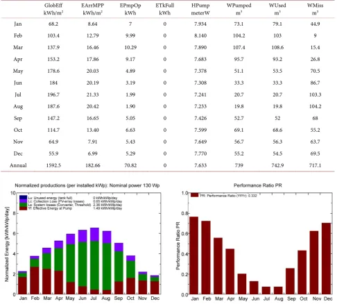
Table 8 represents the numerical simulation results for the PV pumping sys-tem using modules with monocrystalline cells, while Figure 7 shows the norma-lized energy and the performance ratio of the system.

The results show that the system delivered 739 m3 _{of water. There were no} energy losses due to oversizing the system and the overall missing water quantity is of 49.4%. The reason this simulation has a very low yield is due to the fact that the voltage of the PV module (16 V) resides below the converter working voltage (19 - 38 V). Another converter more suited for this system could be installed to obtain better results, however in the PVSyst database, such converter doesn’t ex-ist.

6. Conclusions

Sizing and simulations of a photovoltaic system before installation are a very important step. Critical information could result in finding unknown errors in the system or, why not, enhancing the system overall yield.

This paper shows the results of systems using various solar cell technologies but with almost identical BOS components [15]. For the analyzed systems, our simulations show that polycrystalline solar cell technology offers the best results in terms of overall yield. However, we have to take into consideration that these results are dependent by a series of factors like emplacement, solar resources availability, type of application, operating period, etc., and could differ from other PV application projects in various regions.

Table 8. Monthly numerical simulation results for PV pumping system using modules with monocrystalline silicon cells. GlobEff

kWh/m2 EArrMPP _kWh/m2 EPmpOp _kWh ETkFull _{kWh meterW} HPump WPumped _m3 WUsed _m3 WMiss _m3

Jan 68.2 8.64 7 0 7.934 73.1 79.1 44.9

Feb 103.4 12.79 9.99 0 8.140 104.2 103 9

Mar 137.9 16.46 10.29 0 7.890 107.4 108.6 15.4

Apr 153.2 17.86 9.17 0 7.683 95.7 93.2 26.8

May 178.6 20.03 4.89 0 7.378 51.1 53.5 70.5

Jun 184 20.19 3.19 0 7.308 33.3 33.3 86.7

Jul 196.7 21.33 1.99 0 7.241 20.7 20.7 103.3

Aug 187.6 20.42 1.90 0 7.233 19.8 19.8 104.2

Sep 147.2 16.65 5.05 0 7.426 52.7 52 68

Oct 114.7 13.40 6.63 0 7.599 69.1 68.6 55.2

Nov 64.9 7.91 5.43 0 7.649 56.7 56.3 63.7

Dec 55.9 6.99 5.29 0 7.770 55.2 54.5 69.5

Annual 1592.5 182.66 70.82 0 7.633 739 742.9 717.1

Figure 7. Normalized energy productions, system performance ratio and solar fraction for PV pumping system using

monocrys-talline silicon cells.

should be considered.

References

[1] Mohanty, P., Muneer, T. and KolheSolar, M. (2014) Solar Photovoltaic System Ap-plications. In: Mohanty, P., Muneer, T. and Kolhe, M., Eds., Green Energy and Technology, Springer International Publishing, Switzerland, 49-83.

[2] Wikipedia Contributors (2016) Solar-Powered Pump. https://en.wikipedia.org/wiki/Solar-powered_pump [3] Wikipedia Contributors (2016) Solar Street Light.

https://en.wikipedia.org/wiki/Solar_street_light

[5] Shukla, A.K., Sudhakar, K. and Baredar, P. (2016) Simulation and Performance Analysis of 110 kWp Grid-Connected Photovoltaic System for Residential Building in India: A Comparative Analysis of Various PV Technology. Energy Reports, 2, 82- 88.

[6] Mohammad, B.A., Mahmoud, M.A.V. and Mohsen, M. (2015) Types of Solar Cells and Application. American Journal of Optics and Photonics,3, 94-113.

https://doi.org/10.11648/j.ajop.20150305.17

[7] PVsyst SA (2016). http://www.pvsyst.com/en/about-us [8] Electromagnetica SA (2016).

http://www.elma-led.ro/lampa-stradala-perimetrala-elma-80-12-cu-led#tab-product -view2

[9] Li, J., Wei, W. and Xiang, J. (2012) A Simple Sizing Algorithm for Stand-Alone PV/Wind/Battery Hybrid Microgrids. Energies,5, 5307-5323.

[10] Meteotest (2016).

http://www.meteonorm.com/en/downloads/horizonhttp://files.pvsyst.com/help/sim ulation_variables_standalone.htm

[11] United States Department of Agriculture (2010) Design of Small Photovoltaic (PV) Solar-Powered Water Pump Systems. Technical Note No. 28, Portland, Oregon. https://www.nrcs.usda.gov/Internet/FSE_DOCUMENTS/nrcs142p2_046471.pdf [12] Diaconu, A., Moraru, A. and Fara, L. (2013) PV Pumping Systems. Case Study: Sheep

Farm in South Romania. Proceedings of the International Conference on Energy Efficiency and Agricultural Engineering, Ruse, Bulgaria, 17-18 May 2013, 606-616. [13] PVsyst SA (2016).

http://files.pvsyst.com/help/index.html?simulation_variables_standalone.htm [14] Fara, L., Bartok, B., Moraru, A., Oprea, C., Sterian, P., Diaconu, A. and Fara, S.

(2013) New Results in Forecasting of Photovoltaic Systems Output Based on Solar Radiation Forecasting. Journal of Renewable and Sustainable Energy, 5, Article Num-ber: 041821. https://doi.org/10.1063/1.4819301

[15] Fara, L. and Yamaguchi, M. (2013) Advanced Solar Cell Materials, Technology. IGI Global, Hershey.

Submit or recommend next manuscript to SCIRP and we will provide best service for you:

Accepting pre-submission inquiries through Email, Facebook, LinkedIn, Twitter, etc. A wide selection of journals (inclusive of 9 subjects, more than 200 journals)

Providing 24-hour high-quality service User-friendly online submission system Fair and swift peer-review system

Efficient typesetting and proofreading procedure

Display of the result of downloads and visits, as well as the number of cited articles Maximum dissemination of your research work

Submit your manuscript at: http://papersubmission.scirp.org/