Munich Personal RePEc Archive
Repeated Commuting
Berliant, Marcus
Washington University in St. Louis
18 February 2011
Repeated Commuting
∗
Marcus Berliant
†‡February 2011
Abstract
We examine commuting in a game-theoretic setting with a contin-uum of commuters. Commuters’ home and work locations can be het-erogeneous. The exogenous transport network is arbitrary. Traffic speed is determined by link capacity and by local congestion at a time and place along a link, where local congestion at a time and place is endogenous. After formulating a static model, where consumers choose only routes to work, and a dynamic model, where they also choose de-parture times, we describe and examine existence of Nash equilibrium in both models and show that they differ, so the static model is not a steady state representation of the dynamic model. Then it is shown via the folk theorem that for sufficiently large discount factors the repeated dynamic model has as equilibrium any strategy that is achievable in the one shot game with choice of departure times, including the efficient
∗The author is grateful to David Boyce, whose address at the 2007 Regional Science
As-sociation International North American Meetings in Savannah incited one of his discussants to write this paper. Alex Anas, Richard Arnott, Gilles Duranton, Jan Eeckhout, Eren Inci, Kamhon Kan, Lewis Kornhauser, Bill Neilson, and Ping Wang contributed interesting comments. I am also grateful to seminar audiences at the Public Economic Theory meet-ings in Galway, the Summer Meetmeet-ings of the Econometric Society in Tokyo, the Institute of Economic Research at Kyoto University, the University of Tokyo, and Academia Sinica for comments. Mara Campbell, Tyson King, and Bill Stone of the Missouri Department of Transportation and Lisa Orf of the Missouri State Attorney General’s Office helped me to obtain access to the important and abundant data on St. Louis traffic, useful for detec-tion of equilibrium strategies in the repeated commuting game, and for that I am especially grateful.
†Department of Economics, Washington University, Campus Box 1208, 1 Brookings
Drive, St. Louis, MO 63130-4899 USA. Phone: (314) 935-8486, Fax: (314) 935-4156, e-mail: [email protected]
ones. A similar result holds for the static model. Our results pose a challenge to congestion pricing. Finally, we examine evidence from St. Louis to determine what equilibrium strategies are actually played in the repeated commuting game.
JEL number: R41 Keywords: commuting, folk theorem
1
Introduction
1.1
Motivation
Commuting is a ubiquitous feature of the urban economy. Although the classic literature has answered the basic questions in thefield, such as whether equilibrium commuting patterns are efficient, surprisingly some very important questions remain open. Do models without an explicit (continuous) time clock give us an accurate picture of traffic, in the sense that they can approximate behavior in a truly dynamic model? What happens to commuting when the situation is repeated daily? Does behavior differ dramatically from that observed in the simple context where the commuters know that they only have to commute once? One shot commuting is the exclusive focus of the extant literature.
0 10 20 30 40 50 60
Speed
Speed
[image:3.612.116.489.442.649.2]5 per. Mov. Avg. (Speed)
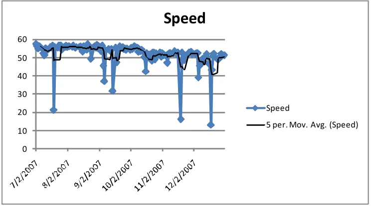
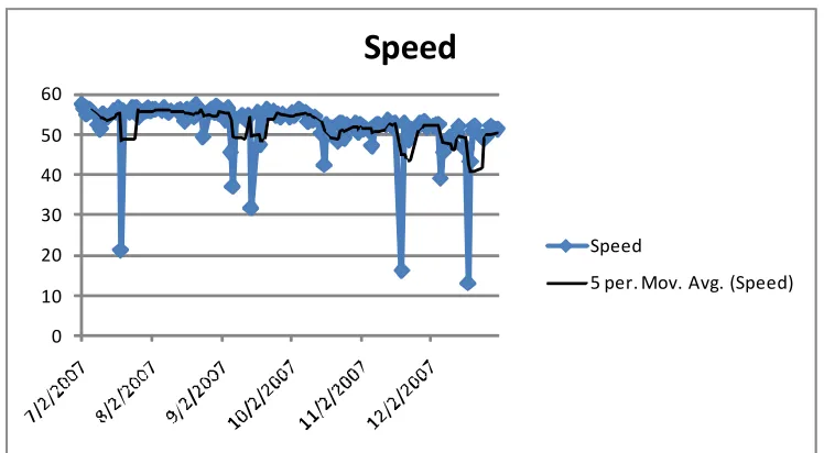
Figure 1: Evening rush hour (5-6 PM) I-64 westbound weekdays .3 miles west of Hampton Avenue
hour traffic speed on the highwaydecrease during the last three months before closure relative to previous dates? We shall return to this in section 3.2 below. But first, we discuss the basic literature on commuting.
Beckmann et al. (1956) provide a model of rush hour where flows are constant. They analyze optimum and equilibrium in a stylized model with no explicit time clock, but with a representative commuter. Vickery (1963, 1969) provided the classical analysis of congestion externalities, pricing, and infrastructure investment. Arnott et al. (1993) examine primarily welfare under various pricing schemes when there is only one route or bottleneck, but allow elastic trip demand and use continuous time. Traffic does not slow down due to congestion, but rather queues at the bottleneck. In their conclusions (p. 177), they note: “In the context of rush hour traffic congestion, for example, models should be developed which derive hypercongestion (traffic-jam situa-tions) from driving behavior, solve for equilibrium on a congested network, and account for heterogeneity among users...” This is what we attempt.
The game-theoretic literature on externalities, for example Sandholm (2001), has the potential to be useful in our context. However, the strong symmetry assumptions used, that yield strong and interesting conclusions, exclude al-most all of the games of interest to us. For example, they exclude the simple special case of our model where there are two nodes called home and work with one link between them, but two departure times. Hu (2010) considers Nash equilibrium with continuous departures for a single commuting corridor for one morning rush hour. It is shown that with a specific dynamic, the equilibrium exists and is unique. As we shall illustrate in the next subsection, multiple equilibria are quite natural in models of commuting. Ross and Yinger (2000) show that the only equilibrium in a general urban equilibrium version of a commuting model with continuous departure times and flow congestion but no bottlenecks is an unreasonable one with a never ending rush hour. As we shall explain below, by allowing a large but finite number of departure times and randomizing departures over small intervals between these discrete depar-ture times, with some effort we can overcome these difficulties. Konishi (2004) considers existence, uniqueness and efficiency of Nash equilibrium primarily in a static model but also in a dynamic model with queues, employing Schmei-dler’s (1973) theorem1 as we do. He uses bottlenecks whereas we use speed
reductions resulting from congestion. Konishi’s work is quite complementary
1To apply Schmeidler’s work to obtain Nash equilibrium in pure strategies, it is important
to ours, as we are not as concerned with the issues he considers, but rather with comparison of equilibria in the static and dynamic models as well as the equilibria of the repeated game.
The transportation engineering literature, for example Daganzo (2008), typically takes the behavior of individuals, namely their choice of routes and departure times, as exogenous. Thus, Nash equilibrium is not studied.2 Once
we have enough notation, we will be specific about how our model compares with its closest relative in that literature.
In summary,the main difference between our work and most of the literature is that we address different questions. That is, our primary purposes are: 1) To compare the Nash equilibria of the one shot commuting games without a time clock to the Nash equilibria of commuting games with a time clock, and 2) To study the equilibria of the commuting game repeated daily. But before considering these issues, first we must prove the basic results involving equilibrium and optimum for our model. A less important difference with much of the literature is that we do not use bottlenecks or queues, instead requiring that traffic slow down as a function of endogenous congestion.
Although the notation used to describe the models formally is burdensome, we will give examples and intuition for the results in addition to the techni-calities. We formulate both a static model, where time plays no role, and a dynamic model, where it does play a role. The dynamic model features a uniform time by which commuters must arrive at work if they don’t want to be subjected to a penalty. We assume that commuters have an inelastic demand for one trip per day to work.
Our results and the outline of the balance of the paper are as follows. In the next subsection of the introduction, we detail and preview our results with minimal notation by using the simplest example, a network with two nodes and one link where all commuters live at one node and commute to their jobs at the other. In Section 2, we give our notation and specify the general static (timeless) and dynamic models. At this point, we also prove our basic results for each model: that Nash equilibria in pure strategies exist, that Pareto optima exist, and that these two sets generally differ. Next, we examine whether the static model can be viewed as a reduced form of the dynamic model, where time is explicit. The answer is an emphatic NO. In Section 3, we study Nash equilibria of each of the models when they are
repeated daily. By applying the folk theorem, wefind that the set of equilibria is much larger than in the one shot game, be it static or dynamic. It is of the utmost importance that researchers consider this expansion of the equilibrium set when analyzing their models. The repeated game structure yields many more equilibria, even when the folk theorem does not apply, than the one shot game structure studied in the literature. Evidence relevant to repeated game strategies used by commuters in St. Louis is examined. Finally, Section 4 gives our conclusions.
1.2
Example
We begin with a simple example to illustrate how the model works and the intuition behind our results. Consider commuters uniformly distributed on the interval [01] with nodes 1 and 2. Each commuter commutes from node
1 to node 2 each day. For simplicity, we only consider the morning rush hour. Denote the capacity of the link by ∈ R+. Suppose that the time
it takes to travel the link at the speed limit is (12) = 1. In the static model, the travel time is given by 1 if the average number of travellers does not exceed capacity of the road, and by 1 otherwise. This means that if road link capacity is exceeded, then traffic slows down in proportion to the ratio of excess commuters to capacity, max(11). For example, if = 12, then the travel time for a commuter on the link is 2. There really are no choices here for the commuters or a social planner optimizing efficiency, since the route is fixed and the model is static; there are no departure times to be chosen.
Now consider a dynamic version of the model. Route choice is stillfixed, but departure (and consequent arrival) times are a choice variable of the com-muters. We model departure times in R+, and we call the required arrival
time at the destination node 2(say 9 AM) ∈R
+. There is no penalty for
The speed of a particular cohort of commuters who depart at the same time is computed as follows. Take the local density of commuters on the road at a particular place on the route and at a particular time. This local density at a given place and time is computed as the limit of neighborhoods on the road of total (measure of) commuters in the neighborhood divided by the one dimensional size of that neighborhood. The limit is taken as the length of the neighborhood goes to zero. The result will be the density of commuters (with respect to distance) at that place and time. Then, as in the static model, traffic slows down in proportion to the ratio of excess commuter density to capacity.
An example will help illustrate. Consider the commuters indexed by[01]. Suppose that all the commuters at 0depart at time 0, all the commuters at 1
depart at time1, and so forth. Set the arrival time= 2. We compute traffic
speeds (in this case, the arrival time does not bind). With these departure times, when road capacity is high so that ≥1, then capacity does not bind. The unit interval of commuters moves from origin to destination at full speed and perfect synchrony, and the local density of traffic is always 1 except for commuters with labels 0 and 1. The density around them is 12 since there is nobody on one side of them (for example the commuters with label 0 have nobody in front of them). But this does not alter their speed, since they are already at the speed limit. In theory, at least, commuters can catch up with those ahead of them (if the ones behind are travelling faster) and slow themselves down.
What if 1? We consider two simple patterns. First, suppose that commuters depart exactly as in the preceding paragraph. Set the arrival time
= 1
+ 1. Traffic slows down by a factor of 1
relative to the no congestion
case; thus, traffic speed for the commuters is uniform at . It takes 1 time to traverse the link, so the last commuters (labelled 1) reach the destination at
1
+ 1. The local density of commuters is 1 during the commute. Call this
the congested commuting pattern.
Now consider the same general departure pattern as in the preceding para-graph, but with commuters labelled 0 beginning travel at time 0, whereas commuters labelled 1begin their trip at time 1. So the density of commuters departing at any time is. Set the arrival time= 1
+1. Since local density
is the same as capacity, all commuters travel at the speed limit. Thus, travel time for all commuters is 1. Call this the uncongested commuting pattern.
illus-trate the computation of local density and speed. Of course, the local density and speed calculations can be much more complicated in, for example, more complicated commuting networks or for more complicated departure patterns. The simple patterns also serve to illustrate the important role played by ar-rival time. It is rather evident that for the fixed arrival time as specified at = 1
+ 1, these strategy profiles are Nash equilibria. Notice that all
commuters reach work by the arrival time for either pattern, but travel
time is longer for the congested commuting pattern. Thus, welfare can differ across dynamic commuting patterns even for this simple example. It is evi-dent that the uncongested commuting pattern Pareto dominates the congested commuting pattern.
Consider next the comparison of the static with the dynamic model. The first pattern, the congested commuting pattern, we study for the case 1
seems to be the analog of the static case, since traffic speed is constricted. But the second pattern does not seem to have an analog. Thus, the static and dynamic models have different Nash equilibrium predictions. Moreover, if the dynamic analog of the static equilibrium is the congested commuting pattern, it is Pareto dominated by another pattern present in the dynamic model but disallowed by the static model.
But we can say more. For example, even in the case where the equilibria of the static and dynamic models appear to be the same, if we average congestion for the dynamic model over time and distances on the link, many times and distances have zero commuters and zero congestion. For instance, this happens at distances along the link in our example that the first commuters have not yet reached. So aggregating the equilibrium of the dynamic model this way will not generate the static model equilibrium, since theflows in the dynamic model will appear diluted.
We return now, and for the remainder of the introduction, to our basic example with 2 nodes and only 1 link. Consider the repeated commuting game for this example. That is, the dynamic commuting game that we have specified is played daily. What payoffs are attainable? We shall apply a folk theorem below, so the set of payoffs attainable as Nash equilibria in the repeated game is related to the payoffs attainable in the one shot game. Specifically, for large enough discount factors in the repeated game, all feasible payoffs at least as high as the maximin payoff for the one shot game (that are not necessarily Nash equilibria of the one shot game) are attainable as Nash equilibria of the repeated game. In fact, we can show that any payoffthat is feasible in the one shot game can be attained as a Nash equilibrium of the repeated game. This result is achieved by simply computing the maximin payoff of the one shot game. It will be−∞. Why? Consider one individual in our simple example. The worst case scenario for that individual in the one shot commuting game is that everyone else who lives at the same node “blockades” them at time zero. That is, the strategy used by everyone else is to depart at time 0. Then local congestion is infinite, so nobody ever reaches the destination or even moves at all, independent of what the commuter in question does (namely, what departure time strategy they follow).3
With the model specified as we have outlined, a Nash equilibrium in pure strategies or an optimum might not exist. So in what follows, for the dy-namic model, we must simplify the problem. This is accomplished by using a fixed, finite set of possible departure times that divide equally the time scale in the model. When commuters choose a departure time, they are distributed uniformly over the interval with midpoint their chosen departure time, and length equal to the distance between allowable departure times. With this structure, a Nash equilibrium in pure strategies and an optimum exist. More-over, the congested and uncongested commuting patterns we have specified are Nash equilibria of the model, and the uncongested commuting pattern is Pareto optimal.
What follows below just makes the ideas behind our simple example formal and general.
3There is an important issue regarding observability or detection of strategies in a model
2
The Commuting Model
Readers who wish to understand the content of the work through examples only can focus on Examples 1-3 below and then skip to section 3.
2.1
The Static Model: Equilibrium and Optimum
Here we lay out the details of a game with an atomless measure space (con-tinuum) of players; a finite set of nodes at which the players live, or to which they commute, or through which they commute; and a finite set of transport links between the nodes with exogenous capacity.
To begin, the measure space of commuters is given by(C ) where is the set of commuters, C is a -algebra on , and is a positive, non-atomic measure.4 We assume that singletons of the form{}for ∈ are inC; that
for all ∈, ({}) = 0; and 0 ()∞.
The origins and destinations in the commuting network are given by a finite set of nodes, denoted by = 12 . Let N = {12 }. The commuting network itself is given by afinite set of links between nodes. The capacity of any direct link (with no intermediate nodes) between nodes and
is given by ∈[0∞], whereas =∞. If a direct link between nodes
anddoes not exist, then = 0.
What remains is to specify the strategies and payoffs of the commuters. In the static game, there is no choice of time of departure or arrival. There is only route choice. To keep the model simple, we shall examine only the morning, not the evening, commute. We assume that each commuter has a fixed origin node and a fixed destination node, with inelastic demand for exactly one trip between the origin and destination. Thus, there is an exogenous, measurable
origin map : → N and an exogenous, measurable destination map : →N.
Aroute for commuter , denoted, is a vector of lengthno less than1but no more than, with()as itsfirst coordinate and()as its last. In other words, is an element of()×[{∅}∪N ∪N2∪· · ·∪N−2]×(). Let
be the map that projects a vector onto its coordinate . Acommuting length map is a measurable map : →{23 }. A commuting route structure
is a pair ( ) where is a commuting length map and is a measurable map : → N() such that almost surely for ∈ ,
1(()) = () and
4Skorokhod’s theorem implies that we could without loss of generality restrict attention
()(()) =().
Given a commuting route structure ( ), its flow ∈ R+2 is given by
( ) = ({ ∈ | ∃ ∈ {12 () − 1} with (()) = and
+1(()) = }) for = 12 . We assume that if a link is
oper-ating below capacity, the time cost of a commuter on that link is constant, call it ( )for = 12 . However, if the link is operating above capac-ity, then the travel time increases in proportion to the excess of commuters above capacity, (()) ·( ).5 For example, if the number of commuters is
twice the capacity of a link, then the travel time is doubled. We ask that the reader bear this special case in mind, since we use it in all of our examples to give concrete intuition.
More generally, we can allow traffic to slow down according to any well-behaved function of the number of commuters at a distance on a link and link capacity. But for simplicity, we specify the function : R+ → R+ where
³(())´yields the rate at which traffic slows in response to congestion. We assume that is strictly increasing and continuous. For our special case,
³(())´≡ (()).
Thetime cost of a commuting structure ( ) for commuter is
( ) =
(X)−1
=1
max(1
µ
((()) +1(()))
((()) +1(()))
¶
)·((()) +1(()))
Thus,−is the objective or payofffunction for each commuter. Theutilitarian welfare function for the static model is
( ) =−
Z
( )()
ANash equilibrium of the static model is a commuting structure( )such that almost surely for ∈ , there is no route of length for commuter
such that
( )
−1
X
=1
max(1
µ
(() +1())
(() +1())
¶
)·(() +1())
5There is an issue of normalization here, namely whether is divided by or not. In
Existence of Nash equilibrium in pure strategies can be proved by applying Schmeidler (1973, Theorems 1 and 2). Rosenthal (1973) proves that a Nash equilibrium in pure strategies exists even when there is a finite number of commuters.
Next we prove (informally) that an optimum exists. The problem can easily be reduced to optimization of the utilitarian welfare function over a compact set as follows. Notice first that there is a finite number of types of commuters, defined by their origin-destination pairs. Instead of using route choice for each commuter, employ as control variables the measure of each type following each route. Thus, the social planner controls a finite number of variables in a compact set using a continuous objective, so a maximum is attained.
Example 1: We note that due to the congestion externality, the Nash equi-libria are unlikely to be Pareto (or utilitarian) optimal. To see this informally, consider an example with 3 nodes. All commuters travel between nodes 1 and 3. There is a direct route, and an alternate route that runs via node 2. The alternative route takes longer than the direct route for each fixed number of commuters below capacity because it requires a longer distance of travel. For example, each road has capacity 1 and takes 1 unit of time to cross, so the longer route uses 2 units of time when running below capacity, whereas the shorter route takes 1 unit of time when running below capacity. Suppose that there is measure 52 of commuters. A Nash equilibrium of this model has the direct route running above capacity, with measure 2 commuters using it for a total travel time of 2, and the indirect route running below capacity (5
measure, with a total travel time of 2) such that the travel time to work for each commuter is the same. To create a Pareto improvement over the Nash equilibrium, simply move some commuters (say measure 5) from the direct to the indirect route. The travel time on the indirect route (namely 2) is the same as at the Nash equilibrium, even for the commuters switched to that route, whereas the travel time for those on the direct route decreases (to15).
2.2
The Dynamic Model: Equilibrium and Optimum
any time ∈ [0 ]. As we shall see shortly, it is important that this set be
bounded. From the list of everyone’s strategies, each commuter can compute with certainty when they will arrive at their destination node.
Adynamic commuting route structure is a triple ( )where : →
[0 ]is a measurable function giving departure times for all commuters, is a commuting length map and is a measurable map : →N() such that
almost surely for ∈, 1(()) =() and()(()) = ().
At this juncture, there is an issue concerning the detail in which we model congestion on each link in the dynamic model. The simplest way to model this is to look only at average congestion on a link. More complicated is to assume that as traffic ebbs and flows, the congestion at the end of the link determines traffic speed on the entire link. The most detailed model, that we use, allows cars to catch up with each other over the course of a link. We use the most detailed model, but assuming link capacity is constant across the link. This is without loss of generality, provided that capacity changes only a finite number of times on a link. In that case, we just add more nodes and links with different capacities.
We shall define commuter progress from origin to destination through a differential equation in distance. But first we must define progress on each component of a route in a dynamic route structure. First,fix a dynamic route structure ( ). The basic idea is this. From departure time to the end
of the first link, we follow the differential equation for congestion for thefirst link, and then begin on the second link, and so forth. Notice that the total distance on a link is given by the distance travelled with no congestion in the minimal time: Z
()
0
1 =( )
This is the length of the link between nodesand. For notational simplicity, for = 1 (), define () to be the time that node (()) is reached.
Evidently, 1() =().
Given a dynamic commuting route structure ( ), we shall associate
with it a function (() ) that gives as its value the distance travelled
on link by commuter at time who begins travel on link at time
(). This function is increasing in its second argument but decreasing in
function . Compute inductively
+1() =
X
=1
()+min{0 0|(())+1(())(()
0) =(
(()) +1(())}
(1) We can then compute its flow at time on link at distance ∆, called
b
:N2×R2
+ →R+. It is given by6
b
( ∆) = lim
→0
({∈ |(() )∈(∆−∆+)})
2 (2)
Then compute
˙
(() ) = min(
1
³( (()))
()
´1) (3)
This describes the progress made by commuters on each link of the entire dynamic commuting route structure for any time .
Unfortunately, as mentioned in Section 1.2 above, the system defining ,
namely (1), (2), and (3), is technically challenging. The reason is that we cannot restrict , the function defining the departure strategies of players,
beyond assuming that it is a measurable function. Each individual makes a choice, and this is not necessarily coordinated. Discontinuities in departure flows or densities can result in discontinuities in ˙ that rule out our ability
to use standard techniques from the theory of ordinary differential equations as well as the contraction mapping theorem. Beyond this issue regarding departure times, there is another factor that comes into play. As we will discuss in detail shortly, if cars can catch up with others on a link (as opposed to at a node), they can slow themselves down by forming an atom; this in itself can cause discontinuities in˙, as it can jump suddenly from a positive
number to zero.7
6The functionbis nothing more than the derivative of the measure induced by . For
more detail, see Rudin (1974, chapter 8), in particular Theorem 8.6.
Even if we can retrieve a well-defined for each function, the issue
then becomes the fact that there might not exist a Nash equilibrium in pure strategies, since the space of pure strategies is a continuum. Schmeidler (1973) relies heavily on the fact that the number of pure strategies available to players is finite.
We solve both of the problems at once by simplifying the dynamic model. Fix small where is an even integer, and define the departure strategy space to be { 3 ( −1)}. This makes the strategy space finite. We assume that all the commuters who choose say will be randomly and uniformly distributed on (02), those who choose the strategy 3 will be randomly and uniformly distributed on (2 4), and so forth. The examples in the introduction and that follow fit this framework because they use a uniform distribution of departure times.
Theorem 1: The system of equations (1), (2), and (3) with initial condition
( ) = 0 for all = 1 and ∈R+ has a unique solution.
Proof: We find the functions and () explicitly. Fix a dynamic
commuting route structure ( ). Let b
( 0) = () +0 where 0 is a
random variable uniformly distributed on (− )denote the actual departure time of commuter , that differs from the chosen departure time () by
at most as described just above. To reduce the notational burden, we shall generally suppress the second argument (0) in any function b. Then
b
1() = b(). In general, given b, we will define inductively b+1. Fix any
origin node and destination node6=. On each segment, defining
() = {0 ∈ |(0) =(); for some ≤(),
1(()) = 1((0)),, −1(()) = −1((0));
−1(()) = −1((0)) =,(()) =((0)) =}
the default speed for commuter is given by
() = min(
1
³(())2
()
´1)
The default speed might be counterfactual, but it is a useful construct. At the default speed, intervals of commuters never overlap with each other. When this happens, the time on this link is exactly ( )(), so b+1() =
b
()+( )()whereas(b() ) =()·[−b()]where(()) =
case is when commuters using different routes blend with each other or sep-arate beginning at a node; this is actually a generalization of the concept of default speed. The third case is if a segment of commuters catches up with another along a link. We consider each of these in turn.
The second case that is possible in the model is when commuters using different routes blend or separate at a node. For the case where they separate, if they are not combined with commuters using other routes, they move at the default speed on the link. But this is just to give intuition. Formally, defining
0( ) ={0 ∈ |0(b−1(0)b())∈((0 )− (0 ));
(()) =, +1(()) =; ((0)) =,+1((0)) =and −1((0)) =0 }
the speed of commuters is given by
∗ () = min( 1
µ
06=lim→0
(0())
()
¶1)
Provided that they don’t catch up with anyone else, their time on the link is ex-actly( )∗ (), sob+1() =b()+( )∗ ()whereas(b() ) =
()·[ −b()] where (()) = . This is actually the most general
form of the speed and time functions. Notice that since the number of types is finite, the denominator of the right hand side of the last equation actually is almost surely constant for sufficiently small.
On each segment , we say that commuter catches up with commuter
0 on link if
(()) =((0)) =, +1(()) =+1((0)) =
b
(0)b()
( ) ∗
()−∗ (0)
b()−b(0)
link, define thecatch up8 time, for
(()) =((0)) =,+1(()) =
+1((0)) =, as ∗ =b() +
∗
(0)·[()−(0)]
∗ ()−∗ (0) . Thus, for all 00 ∈ with
((00)) = , +1((00)) = , b(00) ≥ ∗, then b+1(00) = ∞ whereas
(b(00) ) = (b() ∗) for all ≥b(00) + (()
∗)
∗(00) is constant for
anyone who reaches this spot after the time where the atom forms.
Now that all three cases have been discussed, we can complete the argu-ment. It is essentially a finite but computational argument. Run the entire system, assuming the counterfactual that it always runs at the default speed. This yields a counterfactual solution. Find the first time for which either the second or third case occurs. Now run the entire system again, assuming the default speed except for the deviation caused at this first time. Continue this procedure until all deviations are accounted for. Given the finite nature of the system, this involves only afinite number of times where discrete changes in the system occur. Thus, the algorithm terminates.
Thetime cost of a dynamic commuting structure ( ) for commuter
isR−[b()( )−(()+)]·2·({0∈| 1
1(())=1((0)),2(())=2((0)),()=(0)}).
In essence, this is the expected time cost taken over all commuters using the same pure departure (time and first road) strategy.
We fix an arrival time at ∈ [0∞]. Next we introduce the arrival
penalty function :R+ →R+. To give intuition, think of =()(). The
arrival penalty is given by
()≥0 where() = 0
For example, in the introduction we required that:
Almost surely for∈,b()()≤
Thus, () = 0 for ≤ whereas () = ∞ for . It is actually
more common in the literature to use an asymmetric linear penalty function; see Arnott et al (1993). We can allow further generalization, for example heterogeneous arrival times , but at the cost of messier notation. We note
that in the framework with afinite number of departure times, this is actually the expected penalty for the given choice of strategy, since commuters are randomly assigned over a small interval.
The individual payofffunction for the dynamic model is thus:
− Z
−
[b()( 0)−(() +0) +(b()( 0))]
· 1
2·({0 ∈ |
1(()) =1((0)), 2(()) = 2((0)), () =(0)})
0
Theutilitarian welfare function for the dynamic model is
((·) ) =
− Z
Z
−
[b()( 0)−(() +0) +(b()( 0))]
· 1
2 ·({0 ∈ |
1(()) =1((0)), 2(()) = 2((0)), () =(0)})
0()
ANash equilibrium of the dynamic model is a dynamic commuting structure
( )such that almost surely for∈, there is no route of lengthand
departure time 0 for commuter such that, computing arrival times b0
as in Theorem 1 for the new route and departure time,
Z
−
[b()( 0)−(() +0) +(b()( 0))]
· 1
2 ·({0 ∈ |
1(()) =1((0)), 2(()) = 2((0)), () =(0)})
0
Z
−
[b0( 0)−(0+0) +(b0( 0))]
· 1
2 ·({0 ∈ |
1(()) =1((0)), 2(()) = 2((0)), () =(0)})
0
We note that due to the congestion externality, the Nash equilibria are unlikely to be Pareto (or utilitarian) optimal. Example 2 below will make this precise.
At this point, there is an important but technical issue that must be ad-dressed. One of the requirements of Schmeidler’s results is that utility is continuous (in the weak topology on 1) in the strategy profile of all
atom at that point along the link and comes to a stop. This will hold as long as the second cohort has positive measure. But as we reduce the measure of this second cohort down to zero, it has a very low payoffuntil the limit, where the cohort has zero measure, and catching up with the first cohort does not result in a penalty. In fact the payoff for this zero measure second cohort is larger than for the first cohort, since the second cohort can leave later but arrive at the same time as the first cohort.
Wefix this discontinuity in the obvious way as follows. Any strategy profile that has all strategies used by a positive measure of commuters has its utility for each commuter unchanged. For any strategy profile that has a strategy or strategies used by only a set of measure zero, for each of these strategies we add a set of measure from outside the model using these strategies (leaving the strategies of the commuters in the model unchanged) and define the utility of the limiting strategy to be the limit of the payoffs as → 0. With this modification, payofffunctions are continuous.
Existence of Nash equilibrium in pure strategies can be proved for the version of the model with discrete and finite departure times by ap-plying Schmeidler (1973, Theorems 1 and 2). For the model with a continuum of departure time strategies, we can only obtain existence of -equilibrium in pure strategies.
Similar to the proof for the static model, it is easy to prove that an optimum exists for the discrete departure time model. Instead of looking at a continuum of individual strategies, give the social planner the control variables that are the measure of commuters using each route at each departure time. Given the structure in Theorem 1, the utilitarian objective is upper semicontinuous as a function of the measure of commuters using each route and departure time.9
Example 2: What does Nash Equilibrium look like in the case of a linear penalty function? This is important for applications, as much of the literature uses such a specification. It is actually quite interesting. Suppose that
() =
(
(−) if ≥
( −)if ≥
where , 0. To fix ideas, we consider the example from the introduction, with one link and two nodes, modified for this penalty function. Capacity of the link is= 1, whereas travel time on the uncongested link is1. At a Nash equilibrium, utility must be equalized across commuters, for otherwise everyone
will imitate the happiest ones only. Fortunately for urban economists, this is a familiar condition. There is mass 2 of identical commuters. Consider an example with 2 departure times, 12 and 32. Those who choose departure time 12 actually leave at a random time distributed uniformly between 0 and
1, whereas those who choose departure time 32 actually leave at a random time distributed uniformly between 1 and2. Let = 7
2 and =
1
3. It will
turn out that in Nash equilibrium, the commuters who choose departure time
1
2 travel at the speed limit, whereas the commuters who leave at time 3
2 travel
slower and arrive later. Suppose the (endogenous) measure of commuters who choose departure time 12 is called, whereas the (endogenous) measure of commuters who leave at time 32 is called, where+ = 2. Computing the equal utility condition, for those who choose departure time 12, their travel time is 1 whereas their expected early arrival penalty is 2. For those departing at time 1, their travel time is whereas their expected early arrival penalty is ·(72 −(+ 32)). Setting these negative utilities equal to each other, we obtain = 1−1. Notice that, similar to Example 1, we can create a Pareto improvement by making more agents choose departure time 12. This disrupts the equal utility condition.
Although both Examples 1 and 2 rely on one route or one departure time operating below capacity, this is used only for simplicity. The classical Braess (1968) paradox provides another class of examples. That work shows that in a static model, adding new links to a network can cause equilibrium travel time to increase. For our purposes, the opposite experiment works. If one begins with a network Nash equilibrium and then allows a planner to prohibit travel on some links, a Pareto improvement can be created.
2.3
Can the Static Equilibrium be Supported by a
Dy-namic Equilibrium?
10Here we ask the following question. Given identical exogenous data for the static and dynamic commuting games and finding equilibrium, are the flows in the static and dynamic models the same? This is important for addressing the issue of whether the static model makes sense. For if the answer to this question is negative, then there should be no interest in the static model, since its equilibrium behavior is different from the analogous dynamic model, and the real world is dynamic.
10The ideas in this subsection owe much to Anas (2007) and to discussions with Alex
For simplicity, we return now to the examples used in many of the previous sections, namely where there is no penalty for early arrival and an infinite penalty for late arrival. One could imagine that the static model represents some sort of steady state of the dynamic model, where commuters are intro-duced at constantflows at all the nodes, and theflows in the links are constant over time. But there are two problems with this idea. First, with a fixed ar-rival time (say 9 AM), a steady state does not make sense. The time profile of equilibrium departures will generally not be constant over time, since everyone must get to work by the arrival time. Even if arrival time varied by commuter, one would not expect to see a steady state necessarily attained. Second, the two alternative concepts for consistency of the two models we introduce next are weaker than asking that a steady state of the dynamic model look like a static equilibrium. In other words, if a steady state of the dynamic model looked like the static model, then the conditions would be satisfied. But they are not.
One could ask the question of whether averageflows (over time and space or distance on a link) in the dynamic model are equilibriumflows of the static model. Given the identical exogenous data for the static and dynamic games andfinding equilibrium, does the following condition onflows hold?11
( ) =
R() 0
R
0 ( b ∆) ∆
( )· for all = 12
But this disguises the following issue. In the dynamic model, flows could be high for a time and then zero. The average over the link and over time would be in between, but there would be no actual time and distance on the link where the average was actually attained. So it is logical to ask whether there is a time , and a distance on every link∆( ), such that the flows from the static model are attained by the dynamic model:12
( ) =b( ∆( ))for all = 12
To answer all of these questions in the negative, one only need go back to the simple example with two nodes and one link given in the introduction.
11In a steady state of the dynamic model, this condition would be satisfied because the
flow on each link would be constant, independent of time, and thus be equal to the average
flow.
12In a steady state of the dynamic model, this condition would be satisfied because the
There the uncongested commuting pattern Nash equilibrium is not present for the static model, though the congested one is. But if we want to say something more, for example that there is no equilibrium of the dynamic model that replicates the behavior of the static model, then we must become slightly more sophisticated.
Example 3: We set up a network with 3 identical links in series, each one with the structure of the simple example in the introduction (equivalently, one could use 2 nodes and 1 link with the travel time multiplied by 3). Then if we set the arrival time at 1 + 3(where 1), the congested commuting pattern violates the arrival time for the last commuters, the commuters departing at time 1(they arrive at 3+ 1), and the uncongested commuting pattern remains as the only equilibrium of the dynamic model. It violates all of the conditions above, as there is no uncongested commuting pattern for the static model. In fact, even if we only pay attention to distances on links where there are commuters, their density is 1, never to be found in an equilibrium of the static model. In summary, for this example, the only equilibrium of the static model is the congested commuting pattern, whereas the only equilibrium of the dynamic model is the uncongested commuting pattern. Thus, the equilibrium sets of the two models are unrelated.
3
The Repeated Commuting Game
3.1
The Commuting Folk Theorem and the Commuting
Anti-Folk Theorem
It seems obvious that there are few other games better suited to the folk theo-rem than the (repeated) commuting game, but we have not seen an application. It is not crazy to assume that people play the same game (but not necessarily the same strategy) every day on their commute, modulo random factors such as weather. The folk theorem has proved to be quite robust, so random factors could be added.
of the repeated game. The critical issue in the determination of which one applies is what players observe about other players’ chosen past strategies in finite repetitions of the game. The formalities can get technical; see Kaneko (1982), Massó and Rosenthal (1989), and Massó (1993). So we describe them in a relatively informal manner.
The critical question is this: Afterfinitely many plays of the game,fixing one particular individual, can a positive measure of players observe that indi-vidual player’s behavior? If there is such a set of positive measure for each fixed individual, then the folk theorem applies. Ifno individual’s behavior can be detected by a set of players of positive measure, then the anti-folk theorem applies. Note that these two cases are not exhaustive. In the end, which theorem might apply is an empirical matter. There is some evidence that, in other contexts, the folk theorem is relevant; see, for instance, Lee (1999).
With a finite number of strategies (departure times and routes), it is not far-fetched to think that any particular individual’s strategy is observable by those who use the same departure time and route.13 In the next subsection,
we give a second reason, called the “snowball effect,” why defection from equi-librium strategies might be observable.
Let’s start by assuming observability and apply the folk theorem. Here we examine two repeated games. The first has the static model repeated every day, namely a countable infinity of repetitions. The second has the dynamic model repeated every day. The main results, using Kaneko (1982, Propositions 2.1 and 2.1’), show that if commuters have discount factors suf-ficiently close to one, in other words they do not discount the future much, then there is a huge variety of equilibria. The usual folk theorem holds, so any individually rational, feasible strategy (not necessarily a Nash equilibrium in the one shot game) can be obtained as a Nash equilibrium of the repeated game. Kaneko (1982, Proposition 2.1") proves The Perfect Folk Theorem, where we can restrict even to subgame perfect Nash equilibrium and obtain similar results. The equilibrium strategies are supported by various punish-ment strategies, that apply if the prescribed equilibrium is not followed by a player. Thus, the one day equilibrium is just one of many. Moreover, on the equilibrium path, one only observes the prescribed equilibrium strategies, not the punishments. Thus, one expects to see the one shot equilibrium played, perhaps, but also (for example) the efficient strategies.
13At this point, it is useful to take versions of strategies such that if a set of measure zero
In the static model, the implication is that any feasible route strategy that gives utility at least as high as the maximin payofffor the one shot game for each commuter can be achieved as a constant (over time) Nash equilibrium strategy for the infinitely repeated game with no discounting. If we modify this so that the utility of the strategy in the one shot game is at leastgreater than the maximin utility, then the prescribed strategy can be achieved as a Nash equilibrium strategy in the infinitely repeated game with a discount factor sufficiently close to 1. Example 1 is applicable here. In that example, there is a Pareto improvement where utility is not the same for all commuters. Thus, it will not be a Nash equilibrium for the one shot game, since the commuters with lower utility will try to imitate those with higher utility. However, it can be supported as a (subgame perfect) Nash equilibrium in the repeated game with discount factor sufficiently close to 1. Standard strategies that support this are the threat of Nash reversion.
For the repeated dynamic game, assume that lim→∞() = ∞. One
strategy producing the maximin payoff, equal to −∞ for any commuter, is to blockade the commuter at the first opportunity. If the departure grid is sufficiently fine relative to the measure of commuters departing from each origin node, then other commuters can always make any particular commuter arrive as late as desired. Thus, by choosing the grid to be sufficientlyfine, any payoffis above the maximin payoff. The upshot is that any feasible departure time and route strategy gives a payoffthat is at least as high as the maximin payoff. So any feasible route and departure time strategy for the one shot game can be supported as a Nash equilibrium of the infinitely repeated game without discounting. If we modify this so that the utility of the prescribed strategy in the one shot game is above −∞, then the prescribed strategy can be achieved in the infinitely repeated game with a discount factor sufficiently close to 1. Example 2 is applicable here. In that example, there is a Pareto improvement where utility is not the same for all commuters. Thus, it will not be a Nash equilibrium for the one shot game, since the commuters with lower utility will try to imitate those with higher utility. However, it can be supported as a (subgame perfect) Nash equilibrium in the repeated game with discount factor sufficiently close to 1. Standard strategies that support this are the threat of Nash reversion.
Of course, if no individual’s behavior is observable, then the anti-folk theo-rem applies to both the static and dynamic models, so the only Nash equilibria of the repeated game are the Nash equilibria of the one shot game (Kaneko, 1982, Propositions 2.3 and 2.3’).
3.2
Finite Commuters vs. Continuum of Commuters:
The Snowball E
ff
ect
Here we consider the relevance of models with a continuum of commuters, such as the one we have used. Of course, they are only relevant in the case that they are mathematically convenient approximations to the equilibria of models with a large but finite number of commuters.
With afinite number of commuters, the anti-folk theorem becomes irrele-vant, as the folk theorem applies. With a continuum of commuters without observability of strategies, the anti-folk theorem applies. Due to this apparent discontinuity in the set of equilibria as the number of commuters tends to in-finity, it is imperative to examine the continuity properties of the equilibrium set.
Given the discussion of the previous subsection, we consider two cases in the context of the commuting game: when individual strategies are observable and when individual strategies are unobservable.
When individual strategies are observable, the commuting folk theorem applies to both the model with afinite number of commuters and a continuum of commuters. Thus, there is no issue of a discontinuity as the number of commuters tends to infinity.
these deviations become undetectable, as their effects are small and indistin-guishable from noise. For example, an analog would be to assume perfect competition in the context of a finite number of agents, where the error from this assumption is small for large economies.
If this were true, then there would be no substantial error in simply using the limit commuting game with a continuum of commuters. The big problem here is that the effects of deviations in large butfinite commuting games are not small. To see this, consider the simple example from the introduction with 2 nodes and 1 link. Instead of using a continuum of commuters, consider a large but finite number. Consider either the uncongested or congested commuting pattern. Pure commuter strategies are uniformly distributed over departure times that get the commuters to work by the given arrival time (given that the number of commuters is divisible by the number of such departure times). Suppose that a commuter changes their strategy from the second departure time to the first. This will slow down the first cohort. The second cohort will quickly catch up, slowing down both cohorts. The third cohort will catch up to the first two, and so forth. This “snowball effect” will not only be detectable (even if individual strategies aren’t), but it also substantially changes the behavior of the entire system due to one commuter’s deviation. Such a “snowball effect” is simply not possible in the commuting game with a continuum of commuters.
causes a snowball effect, in that a positive measure of commuters is affected. Then it is assumed that if a positive measure of commuters is affected, this is observable to all and the deviators can be punished.
The problem with this idea is that there is literally no snowball effect with a continuum of commuters, but only with a large but finite (or countable) number. In fact, this is the reason there is a discontinuity of the Nash equilib-rium correspondence in the limit as the number of commuters goes to infinity. A sufficient condition for a snowball effect in large but finite games close to the game with a continuum of commuters of interest is: For the given one shot strategy profile that is to be supported as a repeated game Nash equi-librium, at any time on any link with a positive local density of commuters, local density is above the capacity of the link. Under this condition on the strategy profile, whenever a commuter deviates, there is a snowball effect; this is detected and punished by everyone.
In summary, our conclusion is that although the snowball effect is not present in commuting games with a continuum of commuters, it is present in the large butfinite games nearby. We also assume that effects on any positive measure of commuters are observable to all. Thus, under a sufficient condition on strategies to be supported in the repeated game, it makes sense to say that the consequence of any individual deviation from a prescribed strategy is observable, and thus the folk theorem is applicable to such strategies in the repeated game with a continuum of commuters.
Therefore, be it from observations of neighboring commuters or the snow-ball effect, the folk theorem in the model with a continuum of commuters seems relevant.
A messy alternative to our framework would employ a finite or countable number of commuters and either Nash equilibrium in mixed strategies or -equilibrium in pure strategies. The drawbacks of this approach are tractability and consistency with the balance of the literature on commuting. However, the advantages of this approach are that the snowball effect and application of the folk theorem could be made explicit.
3.3
Evidence
now in the context of commuting.
Consider a repeated game with a termination date that isfinite and known to the players. In general, it is expected that only one shot Nash equilibrium will be played every period, since backward induction leads to the unravelling of other possible equilibrium strategies.
However, as described in Lee (1999, p. 123), there are various theories involving small changes in the classical repeated game model that lead to a kind of folk theorem in finitely repeated games. This is exploited by the empirical work in the field.14 Next we proceed to try to determine which
equilibrium strategy is reflected in commuting data.
If for example the players are myopic and playing one shot Nash, then it is expected that behavior will not change as the termination date approaches. If the players are using strategies other than one shot Nash, for example they are participating in some tacit collusion as the folk theorem might predict, then one expects to see such strategies played when the termination date of the game is not near, but reversion to one shot Nash equilibrium close to the termination date.
How does this work in the context of the repeated commuting game? On January 2, 2008, reconstruction was begun on I-64 (state route 40), a major east-west commuting corridor in St. Louis. A portion was completely shut down. Parts were reopened a year later, though other (adjacent) parts were shut down at that time.15 We take this to be the termination of a repeated,
daily commuting game. This closure was announced years in advance, so it was not a shock to commuters. We examine rush hour traffic speed and volume for locations that were closed on this date.
If commuters were playing one shot Nash strategies, one would expect to see the same rush hour traffic speed daily until close to the closure. Near the time of the closure, traffic would drop off and speed would increase as commuters explored alternate routes to be used after closure.
If commuters were playing a strategy other than one shot Nash, for example Pareto dominant over one shot Nash, then one would expect to see high traffic speed when the closure is not imminent, followed by lower traffic speed as the closure date approaches and one shot Nash is played,16 followed by an increase
14If the folk theorem only applied to infinitely repeated games, those wishing to determine which strategies are played in equilibrium would be waiting a long time for data.
15The entire highway was reopened on December 7, 2009.
in speed near the closure date due to commuters exploring alternate routes.
Thus, it is detection of this counterintuitive decrease in traffic speed as the closure date approaches that can distinguish among the equilibria of the system.
Before presenting the data, it is useful to recall the fundamental identity of traffic, namely: Traffic volume is equal to speed times density. We have obtained data on volume and speed, so density can be calculated. But there are two important points to be made. First, volume is not terribly informative on its own in general, as there can be two equilibria with the same volume, one with low speed and high density, the other with low density and high speed. Second, the externality actually perceived by commuters is in speed, so we focus on that.
We have obtained data from two sensor locations, one toward the east end (closer to the downtown area) of the closure, the other at the west end.17 Let’s
examine the east locationfirst, studying evening then morning rush hour. The figures graph average traffic speed and total volume in the hour by date. We have deleted weekends, but we have not deleted holidays that fall on weekdays.
0 10 20 30 40 50 60
Speed
Speed
5 per. Mov. Avg. (Speed)
Figure 1 (again): Evening rush hour (5-6 PM) I-64 westbound weekdays .3 miles west of Hampton Avenue
17The author was offered more data than the one calendar year at two sensors actually
[image:29.612.115.489.375.581.2]0 500 1000 1500 2000 2500 3000 3500 4000 4500 5000
Volume
Volume
[image:30.612.108.497.78.286.2]5 per. Mov. Avg. (Volume)
Figure 2: Evening rush hour (5-6 PM) I-64 westbound weekdays .3 miles west of Hampton Avenue
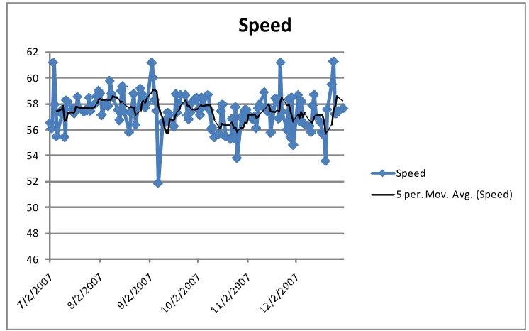
Notice that in early October, there is a decrease in speed and an attendant increase in volume, as seen in Figures 1 and 2. The outliers in the data are obviously accidents. For morning rush hour, as seen in Figure 3, there is a similar effect, though not as large in magnitude and with speed increasing over the Thanksgiving holiday.
46 48 50 52 54 56 58 60 62
Speed
Speed
5 per. Mov. Avg. (Speed)
[image:30.612.114.487.456.689.2]Evening rush hour for the west sensor is displayed in Figure 4. In general, for the west sensor (more distant from the central business district), traffic moves at the speed limit. We conjecture that this is due to the fact that traffic in this area is not congested enough to cause speeds to drop below the speed limit during rush hours.
0 10 20 30 40 50 60 70 80
Speed
Speed
[image:32.612.116.488.75.308.2]5 per. Mov. Avg. (Speed)
Figure 4: Evening rush hour (5-6 PM) I-64 westbound weekdays .7 miles west of Brentwood Boulevard
In summary, there is some evidence that commuters are not playing one shot Nash equilibrium. They revert to one shot Nash strategies at around 2 1/2 to 3 months from the end of the game.
4
Conclusions
in the real world. We have presented some preliminary evidence from the shutdown of an expressway in St. Louis that commuters do not always play one shot Nash equilibrium. We have also discussed the application of the anti-folk theorem to our specific game, namely conditions under which the Nash equilibria of the infinitely repeated game are the Nash equilibria of the one shot game.
The commuting folk theorem poses a direct challenge to congestion pric-ing. If commuters are already playing equilibrium strategies that are efficient without tolls, congestion pricing can mess this up.
The folk theorem and anti-folk theorem can also be applied to repeated versions of other one shot models in the literature, such as Arnott et al. (1993). It would be very interesting to explore experimental complements to our theory and data; for example, see Daniel et el (2009). Which equilibrium of the repeated game is selected in the laboratory?
Future work includes examining the repeated dynamic model with myopic commuters. The set of Nash equilibria will include the equilibria from the one shot game, but not as many as in the repeated commuting game with a discount factor close to 1.
The repeated dynamic model should be applied to real world commut-ing. Since it can accommodate an arbitrary (exogenous) route structure, it has both positive and normative content, especially regarding Pareto improve-ments. For example, it can be used to perform cost benefit analysis with respect to changing infrastructure and mass transit.
References
[1] Anas, A., 2007. “The Trips-to-Flows Riddle in Static Traffic Equilibrium: How to drive a BMW ?” Unpublished manuscript.
[2] Arnott, R., A. de Palma and R. Lindsey, 1993. “A Structural Model of Peak-Period Congestion: A Traffic Bottleneck with Elastic Demand.”
American Economic Review 83, 161-179.
[3] Beckmann, M., C.B. McGuire and C.B. Winsten, 1956. Studies in the Economics of Transportation. Yale University Press: New Haven.
[5] Chung, J.W., 1979. “The Nature of Substitution Between Transport Modes.” Atlantic Economic Journal 7, 40-45.
[6] Daganzo, C.F., 2008. Fundamentals of Transportation and Traffic Oper-ations. Emerald Group Publishing: Bingley, UK.
[7] Daniel, T.E., E.J. Gisches and A. Rapoport, 2009. “Departure Times in Y-Shaped Traffic Networks with Multiple Bottlenecks.” American Eco-nomic Review 99, 2149-2176.
[8] Hu, D., 2010. “Equilibrium and Dynamics of the Discrete Corridor Prob-lem.” Unpublished manuscript.
[9] Kaneko, M., 1982. “Some Remarks on the Folk Theorem in Game The-ory.” Mathematical Social Sciences 3, 281-290.
[10] Konishi, H., 2004. “Uniqueness of User Equilibrium in Transportation Networks with Heterogeneous Commuters.” Transportation Science 38, 315-330.
[11] Lee, I.K., 1999. “Non-Cooperative Tacit Collusion, Complementary Bid-ding and Incumbency Premium.” Review of Industrial Organization 15, 115-134.
[12] Massó, J., 1993. “Undiscounted Equilibrium Payoffs of Repeated Games with a Continuum of Players.” Journal of Mathematical Economics 22, 243-264.
[13] Massó, J., and R.W. Rosenthal, 1989. “More on the ‘Anti-Folk Theo-rem’.” Journal of Mathematical Economics 18, 281-290.
[14] Rosenthal, R.W., 1973. “A Class of Games Possessing Pure-Strategy Nash Equilibria.” International Journal of Game Theory 2, 65-67.
[15] Ross, S.L. and J. Yinger, 2000. “Timing Equilibria in an Urban Model with Congestion.” Journal of Urban Economics 47, 390-413.
[16] Rudin, W., 1974. Real and Complex Analysis. McGraw-Hill: NY.
[17] Sandholm, W.H., 2001. “Potential Games with Continuous Player Sets.”
Journal of Economic Theory 97, 81-108.
[19] Vickrey, W., 1963. “Pricing in Urban and Suburban Transport.” Amer-ican Economic Review 53, 452-465.
[20] Vickrey, W., 1969. “Congestion Theory and Transport Investment.”