Munich Personal RePEc Archive
Development and the cyclicality of
government spending in the Czech
Republic
Szarowska, Irena
Silesian University - School of Business Administration
May 2011
Online at
https://mpra.ub.uni-muenchen.de/32353/
Development and the cyclicality of government spending in
the Czech Republic
Irena Szarowská
1Abstract. This paper aims to provide direct empirical evidence on business cycle re-lations between GDP and government spending in the Czech Republic. Government spending plays an important role in a fiscal policy as a possible automatic stabilizer. We analyzed annual data on government spending in compliance with the COFOG international standard. We use cross-correlation on cyclically filtered adjusted time series over the period 1995-2008. The cyclical properties of GDP and government spending function were, in average, found as weakly correlated. However, we report considerable differences in correlations across the spending functions. The lowest correlation coefficient (0.06) was found for recreation, culture and religion and the highest average was reported for economic affairs (-0.51). As regards to using gov-ernment spending as the stabilizer, total govgov-ernment spending, general public ser-vices, defense, economic affairs and education spending were negative correlated and it confirms countercyclical relation between these spending functions and GDP. It is in line with theory suggestion. On the other hand, the highest spending function (social protection) correlated weak positive and it mean procyclical development.
The results of Johansen cointegration test proved the existence of long-run rela-tionship between GDP and total government spending, public order and safety and economic affairs.
Keywords: government spending, cyclicality, economic growth, correlation, cointe-gration.
JEL Classification: C32, H50, E62
AMS Classification: 90C15
1
Introduction
The economy of the country is greatly influenced by the level and the structure of government spending. The government spending is an important tool for national governments to mitigate the uneven economic develop-ment and economic shocks across individual countries. Governdevelop-ment spending plays important role in a fiscal policy of each country as a possible automatic stabilizer as from a Keynesian perspective, there is a view that government spending should act as a stabilizing force and move in a countercyclical direction. Procyclical fiscal policy is conversely policy expansionary in booms and contractionary in recessions. Serven [13] points that procyclical fiscal policy is generally regarded as potentially damaging for welfare: it can raise macroeconomic volatility, depress investment in real and human capital, hamper growth, and harm the poor. If expansionary fiscal policies in “good times” are not fully offset in “bad times”, they may also produce a large deficit bias and lead to debt unsustainability and eventual default. If a government respect a basic prescription that fiscal tools should function counter-cyclical, the optimal fiscal policy involves a decreasing of government spending in “good times” and a increasing of government spending in “bad times.” Contrary to the theory (it implies that government spending is countercyclical), a number of recent studies found evidence that government spending is procyclical. See Hercowitz and Strawczynski [7], Alesina et al., [2], Rajkumar and Swaroop [12] or Ganeli [4] for more details. Talvi and Vegh [14] show that fiscal procyclicality is evident in a much wider sample of coun-tries. Lane [10] finds procyclicality in a single-country time series study of Irish fiscal policy. As Fiorito and Kollintzas [3] document for G7 countries, the correlation between government consumption and output indeed appears to show no pattern and be clustered around zero. Lane [11] also shows that the level of cyclicality varies across spending categories and across OECD countries. Abbot and Jones [1] test differences in the cyclicality of government spending across functional categories. Their evidence from 20 OECD countries suggests that pro-cyclicality is more likely in smaller functional budgets, but capital spending is more likely to be procyclical for the larger spending categories. Many of researches like Gavin et al. [5], Gavin and Perotti [6] focuse on Latin America. Previously published studies are weakly supported by the data particularly in emerging and post-transition economies in which results can vary. We would like to eliminate the literature gap in this field and analyze government spending in the Czech Republic. The aim of the paper is to provide direct empirical
1
dence on business cycle relation between Gross Domestic Product (GDP) government spending (G) and estimate long-run relationship between these variables in the Czech Republic.
We follow Abbot and Jones [1] and apply the cross-correlation technique and cointegration on annul data of GDP and government spending in compliance with the COFOG international standard during the period 1995-2009 from Eurostat. The paper is organized as follows. In the next section, we describe the dataset and empirical techniques used. In Section 3, we present the results of government spending development and cross-correlation. In Section 4, we estimate long- run relationship between output and government spending. In Section 5, we con-clude with a summary of key findings.
2
Data and Methodology
The dataset consists of annual data on GDP and government spending in compliance with the COFOG interna-tional standard during the period 1995 – 2008. Although data from 2009 are available we prefer to work with a consistent dataset that excludes observations from a crisis period. All the data were collected from the Eurostat database. The series for GDP and total government spending and its subcomponent are adjusted at constant pric-es. We converted all series into logs and applied the Hodrick-Prescott filter with smoothing parameter 100 to each series with the aim to isolate the cycle component of time series. We apply cross-correlation to all combina-tions of GDP – category of government spending. Johansen cointegration test and the error correction model (ECM) are used to estimate the long-run relationship between output and government spending predicted by, for example, Wagner´s Law. Most of the results are calculated in econometric program Eviews 7.
Many studies point out that using non-stationary macroeconomic variable in time series analysis causes supe-riority problems in regression. Thus, a unit root test should precede any empirical study employing such va-riables. We decided to make the decision on the existence of a unit root through Augmented Dickey–Fuller test (ADF test). The equation (1) is formulated for the stationary testing.
t i t k i i t
t
t
x
x
u
x
=
+
+
+
∆
+
∆
− = −∑
1 1 2 10
δ
δ
α
δ
(1)ADF test is used to determine a unit root xtat all variables in the time t. Variable xt-iexpresses the lagged first
difference and ut estimate autocorrelation error. Coefficients δ0, δ1, δ2 and αi are estimated. Zero and the
alterna-tive hypothesis for the existence of a unit root in the xt variable are specified in (2). The result of ADF test,
which confirms the stationary of all time series on the first difference, is available on reguest.
H0: δ2 = 0, Hε: δ2 < 0 (2)
The cross-correlation assesses how one reference time series correlates with another time series, or several other series, as a function of time shift (lag). Consider two series xi and yiwhere i = 0, 1, 2, …, N-1. The cross correlation r at delay d is defined as:
[
]
∑
∑
− − − ∗ − = − − i y d i x i i y d i x i m y m x m y m x r 2 2 ) ) ( ) ( ( ) ( (3)where mxand myare the means of corresponding series.
The Hodrick-Prescott (HP) estimates an unobservable time trend for time series variables. Let yt denote an
observable macroeconomic time series. The HP filter decomposes yt into a nonstationary trend gt and a stationary
residual component ct, that is:
yt = gt + ct (4)
We note that gtand ct are unobservables. Given an adequately chosen, positive value of λ, there is a trend
com-ponent that will minimize:
[
]
∑
∑
= = + − − − − + − T t T t t t t t tt g g g g g
y 1 2 2 1 1 2 ) ( ) ( ) ( min
λ
(5)The first term of the equation is the sum of the squared deviations which penalizes the cyclical component. The second term is a multiple λ of the sum of the squares of the trend component’s second differences. This second term penalizes variations in the growth rate of the trend component. The larger the value of λ, the higher is the penalty. Hodrick and Prescott advise that, for annual data, a value of λ = 100 is reasonable.
The Johansen method [8] applies the maximum likelihood procedure to determine the presence of cointegrat-ing vectors in non-stationary time series as a vector autoregressive (VAR):
t t i t K i i
t
C
x
Z
x
=
+
χ
∆
+
π
+
η
∆
− −=
∑
11
where xt is a vector of non-stationary (in log levels) variables and C is the constant term. The information on
the coefficient matrix between the levels of the Π is decomposed as Π = α β´, where the relevant elements the α
matrix are adjustment coefficients band the β matrix contains the cointegrating vectors. Johansen and Juselius [9] specify two likelihood ratio test statistics to test for the number of cointegrating vectors. The first likelihood ratio statistics for the null hypothesis of exactly r cointegrating vectors against the alternative r +1 vectors is the max-imum eigenvalue statistic. The second statistic for the hypothesis of at most r cointegrating vectors against the alternative is the trace statistic. Critical values for both test statistics are tabulated in Johansen–Juselius [9]. If the variables are non-stationary and are cointegrated, the adequate method to examine the issue of causation is the Error Correction Model (ECM), which is a Vector Autoregressive Model VAR in first differences with the addi-tion of a vector of cointegrating residuals. Thus, this VAR system does not lose long-run informaaddi-tion.
3
Development and the cyclicality of government spending
Government spending can help in overcoming the inefficiencies of the market system in the allocation of eco-nomic resources. It also can help in smoothing out cyclical fluctuations in the economy and influences a level of employment and price stability. Thus, government spending plays a crucial role in the economic growth of a country. We used government spending in compliance with the COFOG international standard (Classification of the Functions of Government) in our analysis. Total government spending is divided into 10 basic divisions:
• G10: General public services
• G20: Defense
• G30: Public order and safety
• G40: Economic affairs
• G50: Environment protection
• G60: Housing and community amenities
• G70: Health
• G80: Recreation; culture and religion
• G90: Education
• G100: Social protection
3.1
The structure of government spending and its development
Firstly we analyzed the structure of government spending in a period 1995-2009. Results in Table 1 show the share of government spending by functions, their average on total spending during the whole period and the share of total government spending on GDP. Data confirm unstable and cyclical development of total govern-ment spending on GDP. In 1995, a high governgovern-ment spending was connected with privatization and transforma-tion process. Five spending functransforma-tions, on average, account for more than 84% of the total spending: social pro-tection, economic affairs, health, general public services and education. Table 1 shows that social protection (G100) was the largest item of government spending from 1996, economics affairs (G40) were on the second and health spending (G70) on the third place till the year 2004. From 2005 the second and the third position has changed.
1995 1996 1997 1998 1999 2000 2001 2002 2003 2004 2005 2006 2007 2008 average
G10 8.1 10.2 9.9 9.3 10 9.9 9.7 10.3 11 10.9 12 10.1 10.2 10.4 10.2
G20 3.4 3.8 3.9 3.5 3.9 4.1 3.6 3.4 4.1 3.1 3.7 2.9 2.8 2.6 3.4
G30 4.8 5.8 5.7 5.1 5.6 5.6 5 4.6 4.7 4.8 4.9 4.9 4.9 4.8 5.1
G40 37 18 19.9 22 19.5 17.5 20.9 19.3 17.6 16.7 15.4 16.2 16.1 16.8 19.3
G50 1.9 2.9 2.6 2.5 2.1 2.2 2.2 2.1 2.4 2.4 2.6 2.6 2.4 2.3 2.3
G60 1.8 2.9 2.5 2.8 2.4 2.6 2.7 1.4 2.6 3.5 3.6 3.6 2.7 2.6 2.7
G70 10.8 14.7 13.5 13.6 13.9 13.7 13.6 13.5 13.5 16.3 16 16.4 16.7 16.8 14.7
G80 2.1 3.1 2.6 2.6 2.4 2.4 2.5 2.7 2.7 2.7 2.7 3.1 2.9 2.9 2.7
G90 7.9 9.7 9.8 9.4 9.4 9.9 9.9 11.1 11 10.7 10.6 11.3 10.9 10.9 10.2
G100 21.9 28.9 29.7 29.2 30.7 32 30.1 31.5 30.3 28.9 28.5 29 30.2 30 29.4
G as %
[image:4.595.75.528.533.710.2]GDP 54.5 42.6 43.2 43.2 42.3 41.8 44.4 46.3 47.3 45.1 45 43.8 42.5 42.9 44.8
Table 1 Development of government spending function
3.2
The cyclicality of government spending
[image:5.595.77.516.136.293.2]As was already noted, government spending is a possible automatic stabilizer. From this point of view, govern-ment spending should move in a countercyclical direction. We decided to assess the relationship between GDP and government spending and we analyzed the correlation between cycle components of GDP and all govern-ment spending functions. Figure 1 shows GDP and total governgovern-ment spending G before and after using HP filter.
Figure 1 Development of GDP and G
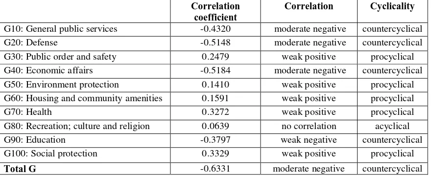
Correlation is a statistical technique that can show whether and how strongly pairs of variables are related. The correlation coefficient can vary from -1 to +1. The correlation coefficient -1 indicates perfect negative corre-lation, and +1 indicates perfect positive correlation. Its value smaller 0.4 means weak correcorre-lation, from 0.4 to 0.7 moderate correlation and higher than 0.7 express strong correlation. A positive correlation coefficient indicates the procyclicality of government spending, negative value means that variables are countercyclical and value close to zero express acyclicality. We run cross-correlations for all possible combinations of GDP and govern-ment spending. The results are reported in Table 2. Here we present coefficients with no lag / lead; all results are available on request.
Correlation coefficient
Correlation Cyclicality
G10: General public services -0.4320 moderate negative countercyclical G20: Defense -0.5148 moderate negative countercyclical G30: Public order and safety 0.2479 weak positive procyclical G40: Economic affairs -0.5184 moderate negative countercyclical G50: Environment protection 0.1410 weak positive procyclical G60: Housing and community amenities 0.1591 weak positive procyclical G70: Health 0.3272 weak positive procyclical G80: Recreation; culture and religion 0.0639 no correlation acyclical G90: Education -0.3797 weak negative countercyclical G100: Social protection 0.3329 weak positive procyclical
Total G -0.6331 moderate negative countercyclical
Table 2 Cyclicality of government spending
The results indicate significant difference across spending functions. We note that 70% of the correlation coefficients are lower than 0.4 in absolute value indicating a weak connection of spending to GDP. Total G, general public services, defense, economic affairs and education were negative correlated and it confirms coun-tercyclical relation between these spending functions and GDP. It is in line with theory recommendation. Con-trary to the theory, the correlation coefficients of the highest spending functions (social protection and health) were weak positive and it reports procyclical development of these sub-categories of government spending and GDP. The lowest correlation coefficient (0.06) was found for recreation, culture and religion and the highest average was reported for economic affairs (-0.51), except the coefficient for total government spending (-0.63).
4
Long- run relationship between government spending and GDP
We also analyzed the long-term relationship between GDP and all government spending functions. The Johansen cointegration test, which is also used in this paper, is nowadays frequently used for testing cointegration. As-sumption for implementation of cointegration is done by the fact that time series are stationary at first difference.
5.7 5.8 5.9 6.0 6.1 6.2 6.3 6.4 6.5
95 96 97 98 99 00 01 02 03 04 05 06 07 08
LGGDP LGG
-.03 -.02 -.01 .00 .01 .02 .03 .04 .05
95 96 97 98 99 00 01 02 03 04 05 06 07 08
[image:5.595.67.508.401.581.2]Individual series are non-stationary, but their common cointegration movement in a long time lead (for example as a result of various market forces) to some equilibrium, though it is possible that in the case of short time periods there is a misalignment of such a long balance. The aim of cointegration test is to determine the number of cointegration relations r in the VAR models. It is also necessary to identify an optimal time lag. The optimal time lag is one period (year) ind it was found with using Akaike information criterion applied to estimation of the non-differenced VAR model. The results of Johansen cointegration test proved the existence of the long-run positive relationship between GDP and total government spending, public order and safety and economic affairs. Findings of test indicated no cointegration between GDP and other spending functions. Cointegration equations have the form expressed in (7), (8) and (9).
∆GDP = 1.083 ∆G – 0.134 (7)
(0.131)*
∆GDP = 1.243 ∆G30 + 0.530 (8)
(0.0226)*
∆GDP = 1.7433 ∆G40 - 2.7241 (9)
(0.2198) *
A symbol ∆ means difference of log variables: GDP, total government spending G, Public order and safety spending G30 and economic affairs spending G40. A symbol * denotes significance at standard 5% level. The above equation shows that increase of total government spending by 1% is connected with increase GDP by 1.08%. We can find similar relationship between GDP and G30 (1.24% ) and GDP and G40 (1.78%).
The cointegration regression considers only the long-run property of the model, and does not deal with the short-run dynamics explicitly. Therefore, ECM is used to detect these fluctuations as it is an adequate tool to examine the short-run deviations necessary to the achievement of long-run balance between the variables. Here, the optimal number of lag is one as was found. We define the ECM for GDP and total government spending in (10) and (11).
∆GDPt = α0 + ω1 (GDPt-1 - γGt-1) + α1∆GDPt-1 + α2∆Gt-1 + u1t, (10)
∆Gt = β0 + ω2 (GDPt-1 - γGt-1) + β1∆GDPt-1 + β2∆Gt-1 + u2t, (11)
In (10) and (11), GDPt and Gt are cointegrated with cointegrating coefficient γ, α0and β0are constants of the
model, ω1 and ω2 note the coefficients of cointegration equition, u1t and u2t mean residual components of
long-term relationship. The ECM equations are similar for G30 and G40 spending functions. The model specification was tested by several residual components tests. We used the autocorrelation LM-test based on Lagranger mul-tipliers, the normality test, and heteroskedasticity test. The performed tests reject the existence of all three phe-nomena. The results of the ECM for all thee founded cointegration are reported in Table 3. Standard errors are in parenthesis.
Cointegration between
Dependent
variable ω1 resp. ω2 GDPt-1 Gt-1 α0 resp. β0
GDP and G
GDPt
-0.0581 0.1661 -0,1389 0.0368* (0.1498) (0.2941) (0.1414) (0.0115) Gt
0.260305 0.2003 -0,0389 0.03599* (0.2122) (0.4165) (0.2003) (0.0163)
GDP and C30
GDPt
-0.5465* -0.0467 0.7594** 0.0346* (0.2353) (0.1878) (0.3348) (0.0092) G30t
1.1608* 0.3390*** -0,0389 -0.0067 (0.3149) (0.2473) (0.2003) (0.0124)
GDP and C40
GDPt
0.0879*** -0.1400 0.0217 0.0330* (0.0524) (0.2493) (0.0337) (0.00826) G40t
0.7623* -0.0153 0.1946*** 0.0281 (0.2167) (1.0311) (0.1405) (0.0342)
Table 3 The error correction models
5
Conclusion
The aim of this paper was to provide direct empirical evidence on business cycle relations between GDP and government spending in the Czech Republic from 1995 to 2009. Government spending plays important role in a fiscal policy as it can help to reduce cyclical fluctuations in the economy.
Although many studies suggest government spending is procyclical despite the recommendations of the theory, our research does not prove that. The results confirm cyclical development of total government spending on GDP in the Czech Republic during 1995-2008. Five spending functions, on average, account for more than 84% of the total spending: social protection, economic affairs, health, general public services and education. The cyclical properties of GDP and government spending function were, in average, found as weakly correlated. However, we report considerable differences in correlations across the spending functions and some correlation coefficients are sufficiently high. The lowest correlation coefficient (0.06) was calculated for recreation, culture and religion and the highest value was reported for economic affairs (-0.51). As regards to using government spending as a stabilizer, total government spending, general public services, defense, economic affairs and edu-cation spending were negative correlated and it confirms countercyclical relation between these spending func-tions and GDP. It is in line with theory suggestion. On the other hand, the highest spending function (social protection) correlated weak positive and it suggests procyclical movement of these spending functions. We also analyzed the long-term relationship between GDP and all government spending functions. The results of Johansen cointegration test proved the existence of long-run positive relationship between GDP and total gov-ernment spending, public order and safety and economic affairs spending functions. As findings verify, they tend to follow GDP and adapt to GDP changes. Tests indicated no cointegration between GDP and other government spending functions.
Acknowledgements
This paper ensued thanks to the support of the grant GAČR 403/11/2073 “Procyclicality of financial markets, asset price bubbles and macroprudential regulation”.
References
[1] Abbott, A., and Jones, P.: Procyclical government spending: Patterns of pressure and prudence in the OECD. Economics Letters111 (2011), 230–232.
[2] Alesina, A. et al.: Why is fiscal policy often procyclical? Journal of the European Economic Association6, no. 5 (2008), 1006–1030.
[3] Fiorito, R., and Kollintzas, T.: Stylized facts of business cycles in the G7 from a real business cycles pers-pective. European Economic Review38 (1994), 235–269.
[4] Ganelli, G.: The International Effects of Government Spending Composition. Economic Modelling27, no. 3 (2010), 631-40.
[5] Gavin, M. et al.: Managing Fiscal Policy in Latin America and the Caribbean: Volatility, Procyclicality, and Limited Creditworthiness. IDB Working Paper No. 326, 1996.
[6] Gavin, M., and Perotti, R.: Fiscal policy in Latin America. Macroeconomics Annual12 (1997), 11–70. [7] Hercowitz, Z., and Strawczynski, M.: Cyclical Ratcheting in Government Spending: Evidence from the
OECD. Review of Economics and Statistics 86, no. 1 (2004), 353-61.
[8] Johansen, S.: Cointegration and Hypothesis Testing of Cointegration Vectors in Gaussian Vector Autore-gressive Models. Econometrica 59, no.6 (1991), 1551–1580.
[9] Johansen, S. and Juselius, K.: (1990): Maximum Likelihood Estimation and Inference on Cointegration, with Applications. Oxford Bulletin of Economics and Statistics 52 (1990), 169–210.
[10]Lane, P. R.: International Perspectives on the Irish Economy. Economic and Social Review 29, no. 2 (1998), 217-22.
[11]Lane, P. R.: The Cyclical Behaviour of Fiscal Policy: Evidence from the OECD. Journal of Public Eco-nomics 87, no. 12 (2003), 2661-75.
[12]Rajkumar, A. S., and Swaroop, V.: Public Spending and Outcomes: Does Governance Matter? Journal of Development Economics 86, no. 1 (2008), 96-111.
[13]Serven, L. Macroeconomic Uncertainty and Private Investment in LDCs: an Empirical Investigation. World Bank Working Paper No. 2035, 1998.