Munich Personal RePEc Archive
Longevity, life-cycle behavior and
pension reform
Haan, Peter and Prowse, Victoria
Cornell University, Department of Economics, DIW Berlin - German
Institute for Economic Research
6 June 2012
Longevity, Life-cycle Behavior and Pension Reform
Peter Haan∗, Victoria Prowse†
June 6, 2012
Abstract
How can public pension systems be reformed to ensure fiscal stability in the face of in-creasing life expectancy? To address this pressing open question in public finance, we use micro data to estimate a structural life-cycle model of individuals’ employment, retirement and consumption decisions. Our modeling approach allows life expectancy and the nature of the public pension system to influence the decisions of forward-looking individuals planning for retirement. We calculate that, in the case of Germany, an increase of 4.34 years in the full pensionable age or a cut of 37.7% in the per-year value of public pension benefits would offset the fiscal consequences of the 6.4 year increase in age 65 life expectancy anticipated to occur over the next 40 years. Of these two approaches to coping with the fiscal impact of improving longevity, increasing the full pensionable age generates the largest responses in labor supply and retirement behavior.
Keywords: Life Expectancy; Public Pension Reform; Retirement; Employment; Life-cycle Models; Consumption; Tax and Transfer System.
JEL Classification: D91; J11; J22; J26; J64.
∗DIW Berlin, [email protected]
1
Introduction
Over the last several decades the longevity of individuals living in the developed world has im-proved considerably and consistently, and this trend looks set to continue.1 Such a demographic change poses numerous social and economic challenges. Notably, many public pension systems, which are typically compulsory defined benefit schemes, are being strained by the greater pen-sion demands concurrent higher life expectancy. In response to this problem, an important political debate has arisen concerning how to reform public pension systems to address the fis-cal demands created by improving longevity. This debate has focused on identifying effective ways of increasing the age-based eligibility requirements associated with public pension benefits. The policy response thus far has reflected this theme: for example, Germany and the US have recently announced plans to gradually increase the full pensionable age, that is the age from which an individual may claim a non-reduced public pension, from 65 to 67 years.
We use a comprehensive dynamic structural model to understand the relationship between life expectancy, the public pension system and individuals’ employment, retirement and con-sumption decisions over the life-cycle. We use the Method of Simulated Moments to estimate the model’s parameters. Drawing on this framework, we are the first to analyze how changes in life expectancy affect optimal individual employment, retirement and consumption through the life-cycle. By looking at how individuals respond to changes in individual and cohort-specific longevity, we break new ground by exploring the desirability of changes in the public pension system designed to cope with the fiscal challenges posed by increasing life expectancy. This paper therefore makes a novel contribution to the policy debate on how public pension systems can be reformed to deal effectively with the consequences for Government finances of increasing life expectancy.
Our structural life-cycle model includes stochastic job offers, involuntary separations, saving opportunities and borrowing constraints, early retirement possibilities, unobserved heterogene-ity in preferences, employment opportunities and wages, and detailed specifications of the tax and transfer systems. Moreover, the modeling approach naturally allows life expectancy and the public pension system to influence the decisions of forward-looking individuals planning for retirement. This methodology is ideally suited to quantifying the effect of life expectancy on behavior and to exploring the consequences of reductions in public pension generosity. By considering the interplay between life expectancy and public pension reform when individuals may adjust employment, retirement and consumption behavior, we expand on previous ap-plications of structural life-cycle models. In particular, our paper builds on several previous structural studies which have used life-cycle models to investigate the effects of public pension systems on labor supply, retirement and consumption decisions (e.g., Casanova, 2010, French, 2005, French and Jones, 2011, Gustman and Steinmeier, 1986, Gustman and Steinmeier, 2005, Heyma, 2004, Jim´enez-Mart´ın and Sanchez Mart´ın, 2007, Rust and Phelan, 1997, and van der Klaauw and Wolpin, 2008) and on work that developed structural life-cycle models in which in-dividuals choose jointly consumption and labor supply (e.g., Imai and Keane, 2004, and Keane
1E.g., Oeppen and Vaupel (2002) show that over the last 150 years life expectancy at birth in the developed
and Wolpin, 2001).2 Our paper is also related to a small literature that looks at the effect of life expectancy on the saving decision alone (see Brown, 2001, De Nardi et al., 2010, Gan et al., 2004, and Hurd, 1989).
We implement our model in the context of Germany, a country with a compulsory pay-as-you-go defined benefit public pension system which displays many similarities to Social Security in the United States. Couching the analysis in the context of Germany allows us to exploit a unique pattern of variation in the evolution of demographic group-specific life expectancy which arose due to events that followed German reunification in 1990. Specifically, drawing on variation between demographic groups in the extent of improvements in life expectancy, we demonstrate that the estimated model predicts the observed relationship between life expectancy and retire-ment. This suggests that our model provides a sound basis for counterfactual policy simulations which explore the effect of life expectancy on employment, retirement and consumption behavior. In terms of data sources, we obtain projections of age-specific life expectancies by cohort, region and gender from the Human Mortality Database for Germany. Data on life expectancy are combined with a sample of older individuals taken from the German Socio-Economic Panel and covering the years 1991 - 2007. In addition to replicating the observed relationship between life expectancy and retirement behavior as discussed above, the fitted model is able to reproduce the distribution of observed wages, the age profile of wealth and the age-specific rates of transitions between employment and unemployment.
The leading results of counterfactual simulations based on the estimated structural life-cycle model are twofold. First, in response to an increase in life expectancy we find that individuals work more and postpone retirement, and thereby increase public pension benefits for their now longer retirement periods. Reflecting this behavioral adjustment, an increase in life expectancy leads to higher net Government revenues received from individuals aged below the full pension-able age; however, the increase in net revenue from individuals aged below the full pensionpension-able age is dwarfed by the increase in public pension demands. Qualitatively, the 6.4 year increase in age 65 life expectancy anticipated to occur over the next 40 years leads average net Government revenue per person, summed over the life-cycle starting at age 40 years and continuing until death, to decrease by approximately 75000 Euros.
Second, we demonstrate striking differences between behavioral responses to two revenue equivalent reductions in public pension generosity. We calculate that the fiscal consequences of the 6.4 year increase in age 65 life expectancy anticipated to occur over the next 40 years can be offset by either an increase of 4.34 years in the full pensionable age or a cut of 37.7% in the per-year value of public pension benefits. We find that the increase in the full pensionable age elicits a marked increase in the employment rate, while a revenue equivalent the cut in the per-year value of public pension benefits has little impact on employment outcomes. Intuitively, the increase in the employment rate associated with the increase in the full pensionable age arises because the age-based eligibility rules embedded in the public pension system represent binding constraints on access to public pension benefits for many individuals. Meanwhile, those
2A largely separate literature presents empirical evidence from micro data of a direct effect of pension rights
individuals most affected by a cut in the per-year value of public pension benefits are likely to be in employment and ineligible for early retirement, and hence are generally unable to increase employment. We compute that expected total per-person post age 40 years consumption is over 100000 Euros higher if the fiscal consequences for the Government of 40 years worth of improvements in longevity are counteracted by an increase in the full pensionable age rather than a revenue equivalent cut in the per-year value of pension benefits.
This paper proceeds as follows. Section 2 outlines our life-cycle model. Section 3 describes our data sources. Section 4 provides an overview the estimation methodology, presents our structural parameter estimates and demonstrates the model’s goodness of fit. Section 5 discusses the results of counterfactual policy simulations. Finally, Section 6 concludes.
2
Model
2.1 Overview
To examine the impact of life expectancy on life-cycle behavior and to explore the effectiveness of public pension reforms, we develop a rich dynamic structural model of individual’s employ-ment, retirement and consumption decisions over the life-cycle. We propose a discrete-time finite-horizon model. Each quarter, i.e., every three months, an individual chooses his or her current labor market state and current consumption.3 We distinguish three labor market states: full-time work (f); unemployment (u); and retirement (r).4 Retirement is an absorbing state. Individuals are indexed by i= 1, ..., N, and age, measured in quarters of a year, is indexed by t.5 The maximum possible age to which an individual can live is denoted byT. We follow the life tables and use T = 110 years. We focus on the employment, retirement and consumption behavior of individuals aged 40-65 years. Following De Nardi et al. (2010), in the interest of ensuring that our empirical analysis captures precisely the relevant institutional and environ-mental factors we study only those individuals who reside in single-adult households and who do not have dependent children.6
Each period, an individual enjoys a flow of utility which depends on current consumption, ci,t, current leisure and individual-specific preference shifters. We use Ui,t(ci,t, j) forj =f, u, r to denote individual i’s age t flow utility from state j. Following Low et al. (2010), we adopt
3Quarterly decision making allows accurate modeling of the Unemployment Insurance system.
4Full-time work is 39 hours of work per week. This is the median hours of work of sampled individuals.
5To improve readability we do not introduce further subscripts to index specific cohorts or years: cohort
information is specific to the individual, and together with age information, the year is thereby defined.
6Older non-retired individuals constitute the demographic group for which we expect that behavior is most
the following constant relative risk aversion (CRRA) specification for preferences:
Ui,t(ci,t, f) = β(ci,t(1−ηi)) 1−ρ
1−ρ +εi,f,t, (1)
Ui,t(ci,t, j) = β c1i,t−ρ
1−ρ +εi,j,t for j=u, r. (2)
In equations (1) and (2),ρis the coefficient of relative risk aversion, andηidescribes the comple-mentarity between consumption and leisure. We imposeηi∈[0,1), and this has two implications. First, we can interpret ηi as the share of consumption necessary to compensate individual ifor the disutility of working. Second, consumption and leisure are Frisch complements, meaning that,ceteris paribus, the marginal utility of consumption is higher for working individuals than for either unemployed individuals or retired individuals. We allow unobserved heterogeneity in the complementarity between leisure and consumption by assuming that ηi|χi ∼ N(µη, ση2), where χi denotes the individual’s observed characteristics at the time of labor market entry.7 The unobservablesεi,f,t,εi,u,t and εi,r,t represent transient individual-specific preference shifters while the parameter β determines the importance of consumption and leisure in preferences, relative to the transient individual-specific unobservables.8,9
Current consumption is the sum of current net income and current dissaving. Current net income depends on the individual’s gross incomes from employment and from interest on wealth, and on the contemporaneous tax, transfer and pension systems. Our model includes an accurate representation of the tax system, including income tax deductions and Social Security Contributions. The model also includes the two leading forms of out-of-work transfers: Social Assistance; and Unemployment Insurance. Appendix E provides further information about the tax and transfer systems. Further details about the modeling of the pension system can be found in Section 2.4.10
7To guarantee thatη
i∈[0,1) we truncateηifrom above at 0.999 and from below at zero. According to this
specification, preference heterogeneity occurs independently of observed individual characteristics at the time of labor market entry. However, due to the endogenous accumulation of experience and wealth occurring within the model, preference heterogeneity will correlated with observed individual characteristics at dates subsequent to labor market entry. We will estimate the model directly and therefore our empirical analysis accounts fully for such processes.
8Theεs are assumed to occur independently over individuals. Theεs for individualiare assumed to occur independently over time and over the labor market statesj=f, u, r. Further, the individual’s aget εs are assumed to be independent of the individual’s agetobserved characteristics. Additionally,εi,j,tfor alli,jandtis assumed
to have a type I extreme value distribution. The inclusion of this form of unobservables in the flow utilities has the effect of smoothing the value function and thus facilitates estimation of the structural parameters.
9The utility function described by equations (1) and (2) is a minor generalization of a Cobb-Douglas utility
function: Equations (1) and (2) can be rewritten as
Ui,t(ci,t, j) = c1i,t−ρL ρ
i,j+ϵi,j,t for j=f, u, r, (3)
whereϵi,j,t=β−1(1−ρ)εi,j,tandLi,j= (1−ηiHj)(1−ρ)/ρwhereHjrepresents the percentage of full-time working
hours spent in employment in statej(for the labor market states appearing in our model we haveHu=Hr= 0
andHf = 1).
10The German tax, transfer and pension systems were subject to several reforms during the sample period. We
Individuals are forward-looking and each period make employment, retirement and con-sumption decisions to maximize the discounted expected value of future utility. An individual’s optimization problem age tis given by
max d,c Et
T
∑
s=t
δs−tki,s,tUi,s(ci,s, di,s). (4)
In the above di,t ∈ {f, u, r} is a categorial variable which codes the individual’s age t labor supply and retirement behavior. The variable ddetails the individual’s employment and retire-ment behavior in each remaining period of the individual’s life. Similarly, c is a vector that describes the individual’s consumption choice in each remaining period of the individual’s life. The operatorEt is an expectation conditional on the individual’s agetinformation set. Payoffs occurring in the future are discounted due to subjective time discounting and mortality risk; δ ∈ [0,1] is the subjective time discount factor, and ki,s,t is the probability of the individual surviving until age sconditional on being aged t.
The inclusion of survival probabilities in the individual’s objective function reflects the de-pendence of life-cycle utility on life expectancy. We follow, inter alios, De Nardi et al. (2010), van der Klaauw and Wolpin (2008) and Rust and Phelan (1997) and allow individual-level het-erogeneity in life expectancy. Specifically, we allow variation in survival rates, and therefore life expectancy, according to gender and region of residence. Additionally, extending on previous studies, we allow life expectancy to be cohort-specific and therefore we capture the sizable im-provements in life expectancy that have occurred in recent years. In Section 3.2 we discuss the empirical relevance and statistical advantages associated with our relatively rich approach to modeling life expectancy.
The optimization process is subject to an intertemporal budget constraint. In addition, behavior is subject to constraints on borrowing and on the availability of employment and re-tirement opportunities. We describe below: (i) the processes that determine job offers and involuntary separations and thereby dictate employment opportunities; (ii) the composition of gross wage income; (iii) public pension benefits and early retirement opportunities; (iv) borrow-ing constraints, consumption possibilities and the intertemporal budget constraint; and (v) the optimal arrangement of employment, retirement and consumption over the life-cycle.
2.2 Employment Opportunities
An individual’s behavior is constrained by the availability of employment opportunities (see Blundell et al., 1987, and Blundell et al., 1998, for discussion of labor supply rationing). Ra-tioning of labor supply is an important life-cycle phenomena: it contributes to prolonged periods of unemployment and therefore affects retirement incentives when public pension benefits are linked to life-time labor market outcomes.
Employment opportunities are modeled as follows. Each period an unemployed individual receives a job offer with probability Θi,t. Upon receipt of a job offer, the individual observes the current gross wage, wi,t, associated with the job opportunity. The age t job offer probability takes the form
Here and henceforth Φ() denotes the cumulative distribution function of a standard normal random variable. We allow the job offer probability to depend on age, region of residence and health status, and variables measuring these characteristics are included inxi,t. λΘ is a suitably dimensioned parameter vector. Finally,µΘ
i represents unobserved individual characteristics. An individual in receipt of a job offer has the option of moving into employment in the current period. With probability (1−Θi,t) a previously unemployed individual does not receive a job offer at age t, in which case a transition into employment in the current period is impossible.
Similarly, each period an employed individual experiences an involuntary separation with probability Γi,t. The age tprobability of an involuntary separation takes the form
Γi,t = Φ(λΓxi,t+µΓi), (6)
whereλΓ is a suitably dimensioned parameter vector andµΓ
i is an unobserved individual effect. An individual subject to an involuntary separation does not have the option of remaining in employment in the current period. With probability (1−Γi,t) a previously employed individual does not experience an involuntary separation and has the opportunity to stay in employment and to be paid new gross wage, wi,t.
We interpret the unobserved individual effects that appear in the job offer and involuntary separation probabilities as permanent unobserved individual characteristics that impact on an individual’s ability to find or keep a job. These unobservables are assumed to be assigned to an individual at the time of first labor market entry. The joint distribution of the unobserved individual effects is given by [µΘ
i , µΓi]|χi∼N(0,Σµ).
2.3 Gross Wage Offers
Gross wage income in an important component of current and future financial incentives. There-fore, we adopt the following rich specification for offered gross hourly wages
log(wi,t) =λzi,t+αi+τi,t+υi,t. (7)
In the above, zi,t contains observed individual characteristics including education, region of residence and experience, and λ is a suitably dimensioned parameter vector. The inclusion of experience is important here because it captures the endogenous accumulation of experience-based human capital (e.g., Eckstein and Wolpin, 1989, and Keane and Wolpin, 1997).
The final three terms in the wage equation are the unobserved components of wages. αi is a permanent individual-specific random effect, representing ability or skill. We take αi to be assigned to an individual at the time of first labor market entry and assume αi|χi ∼N(0, σ2
α). τi,t is a persistent unobservable, which we interpret as an employer-employee match-specific pro-ductivity effect. For an individual who was employed in the previous period,τi,t keeps the same value as in the previous period with probability Π, and with probability (1−Π) the individual’s match-specific productivity is subject to a shock. In the latter case, the individual receives a new match-specific productive effect τi,t|ϕi,t ∼N(0, σ2
offer in the current period receives a new match-specific productivity shock τi,t|ϕi,t ∼N(0, στ2). In contrast to Low et al. (2010), we do not model or observe transitions between employers; we identify Π and σ2
τ from the persistence in individual-specific wage observations (see Table 6). Finally, υi,t|ϕi,t ∼N(0, σ2
υ) is a transitory wage shock. The parameters of the wage process are estimated jointly with the other structural parameters (see Section 4.1).11
2.4 Public Pension Benefits and Early Retirement Opportunities
Similar to many public pension systems, German public pension benefits reflect an individual’s employment and earnings outcomes prior to retirement, and this linkage works to strengthen the interplay between life expectancy, the public pension system and life-cycle behavior. We provide here an overview of the relevant aspects of the German public pension system. Unless noted otherwise, the model is estimated with the specification of pension benefits described below. Further details can be found in Appendix F.12
Public pension benefits in Germany are linked to an individual’s labor market history via a quantity we refer to as “weighted pension points”. An individual accumulates one pension point for every year of employment and such pension points attract a weight of min{wi,t/wi,t, M axi,t}, where wi,t denotes the mean gross wage in the period when individual i is age t and M axi,t denotes the year-specific cap on pension point weights. During the sample period, the cap on pension point weights was roughly equal to two in all years. An individual also accumulates one pension point for every year of Unemployment Insurance-eligible unemployment. Such pension points are allocated a weight of min{0.8×wi,t′/wi,t,0.8×M axi,t}, where t′ denotes the age at which the individual was last employed. Thus, up to a cap of roughly 1.6, an unemployed individual’s pension points are weighed by the ratio of 80% of the individual’s most recent gross wage relative to the current mean gross wage.
Age-based criteria govern access to public pension benefits and the generosity of public pension benefits. Arguably the most important age-based parameter is the full pensionable age. At this age, which is 65 years for the individuals under study, an individual can retire and receive a publicly provided pension with a value proportional to the sum of weighted pension points accumulated prior to retirement. The German public pension system is relatively generous: according to B¨orsch-Supan and Schnabel (1998), in 1998 public pension benefits provided a replacement rate of around 70% of pre-retirement net earnings for an individual retiring at the full pensionable age with 45 years of working experience and average life-time earnings.
The public pension system offers numerous opportunities for retirement prior to the full pensionable age and our model captures most important routes into early retirement. Specif-ically, our model recognizes that an individual may be eligible for retirement prior to the full pensionable age on the grounds of: (i) gender, specifically being a woman; (ii) disability; or (iii) working history, specifically having previously worked at least 35 years. Eligibility for early
11At all ages the three unobserved components of wages are assumed to be mutually independent and
indepen-dent of the unobservables [µΘi, µΓi] that affect the job offer and involuntary separation probabilities.
12B¨orsch-Supan and Wilke (2004) note that the public pension system in Germany accounts for approximately
retirement on the grounds of gender or working history is dependant on the individual’s age (e.g., only those who have worked at least 35 years may retire from age 63 years). The age, gender and working history-based eligibility criteria for early retirement are entirely objective and the relevant rules are hard-coded into the model. When doing this, we account fully for intertemporal variation in the early retirement eligibility criteria. In contrast, the rules that determine eligibility for public pension benefits on the grounds of disability are complex and the operationalization of these rules has inevitably been somewhat subjective. For the purpose of implementing our model, we assume that individualihas a probability Υi,t of being eligible, due to disability, for early retirement. The aget probability of being eligible for public pension benefits on the grounds of disability is as follows
Υi,t = Φ(λΥqi,t), (8)
whereqi,t contains variables that measure the individual’s gender and health status, andλΥ is a suitably dimensioned parameter vector. The per-year value of public pension for an individual taking early retirement depends on the year-specific legislation, gender, disability status, working history and age. Appendix F.3 provides further details.
2.5 Borrowing, Consumption and the Intertemporal Budget Constraint
Individuals may save and borrow. Wealth (Wi,t) here refers to an individual’s private wealth holdings, and therefore excludes the value of any entitlements to the public pension or other social programs. The individual faces borrowing constraints which restrict wealth to be non-negative, that is Wi,t ≥0. This assumption, which follows French (2005) and Low et al. (2010), reflects that borrowing typically requires collateral and that individuals are unable to borrow against future earnings or future Unemployment Insurance, Social Assistance or public pension benefits.
Subject to the above-described borrowing constraint, each period, a non-retired individual chooses a consumption level, ci,t. Quarter-by-quarter wealth accumulation for a non-retired individual is described by the following intertemporal budget constraint
Wi,t+0.25=Wi,t+ 1(di,t =f)mi,f,t+ 1(di,t =u)mi,u,t−ci,t. (9)
In the above mi,f,t and mi,u,t are the net incomes that arise from full-time employment and unemployment. (These net incomes are determined by the tax and transfer systems, gross wage income and income from wealth - see Appendix E). Note that, given consumption behavior, wealth accumulation depends on the real interest as the net incomesmi,f,tandmi,u,tinclude the net-of-tax value of interest income. In contrast to the models of retirement behavior developed by, e.g., French and Jones (2011) and Rust and Phelan (1997), we do not include medical expenses. This is reasonable because Germany has a universal health care system.
We assume that a retired individual’s consumption is consistent with the actuarially fair annuity value of accumulated wealth. The per-period consumption enjoyed by an individual who retires at age tthus given by
whereai,t denotes per-period annuity value of wealth for an individual who retires at aget. This specification captures the primary intertemporal incentives important for the current application. In particular: (i) wealth accumulation prior to retirement is valuable in retirement; (ii) the value of accumulated wealth is negatively related to life expectancy (as the actuarially fair annuity value of wealth depends negatively on life expectancy); and (iii) financing consumption out of accumulated wealth is a substitute for funding consumption from public pension benefits.
2.6 Optimal Labor Supply, Retirement and Consumption
2.6.1 Solution Method
Drawing on dynamic programming techniques, we use our model to describe an individual’s op-timal employment, retirement and consumption behavior over the life-cycle. An individual’s age t optimization problem can be expressed in terms of the state-specific value functionsVtj,c(pi,t) forj =f, u, r, which define the maximized discounted expected value of the individual’s future life-cycle utility conditional on being in statej with current consumption ofc. Here,pi,t denotes the timet values of the state variables for individuali.13 Using ˇtto denote the individual’s age in the next quarter, i.e., ˇt≡t+ 0.25, the state-specific value functions are defined recursively as follows
Vtf,c(pi,t) = Ui,t(c, f) +δki,ˇt,tEt
[
Γi,tˇ
{
Λi,ˇtmax{Vtˇu(pi,ˇt), Vˇtr(pi,ˇt)}+ (1−Λi,ˇt)Vˇtu(pi,ˇt)
}
+
(1−Γi,ˇt)
{
Λi,ˇtmax{Vˇtf(pi,ˇt), Vtˇu(pi,ˇt), Vˇtr(pi,ˇt)}+ (1−Λi,ˇt) max{Vtˇf(pi,ˇt), Vˇtu(pi,tˇ)}
}]
,(11)
Vtu,c(pi,t) = Ui,t(c, u) +δki,t,tˇ Et
[
(1−Θi,ˇt)
{
Λi,ˇtmax{Vtˇu(pi,ˇt), Vˇtr(pi,ˇt)}+ (1−Λˇt)Vˇtu(pi,ˇt)
}
+
Θi,ˇt{Λi,ˇtmax{Vˇtf(pi,ˇt), Vˇtu(pi,ˇt), Vtˇr(pi,tˇ)}+ (1−Λi,ˇt) max{Vtˇf(pi,ˇt), Vtˇu(pi,ˇt)}}
]
, (12)
Vtr(pi,t) = Ui,t(cri,t, r) +δki,t,tˇ EtVˇtr(pi,tˇ). (13)
In (11)-(13) above, Λi,ˇtis the individual’s probability of being eligible for retirement at age ˇt.14 Meanwhile, Vi,fˇt(pi,ˇt) and Vi,uˇt(pi,ˇt) are defined as the age ˇt value functions associated with age ˇ
t employment and unemployment, respectively, after age ˇt consumption has been optimized. Specifically,
Vi,jtˇ(pi,ˇt) = max
c V
j,c
i,ˇt (pi,tˇ) for j=f, u. (15)
13The state variable are: W; q; µΘ; µΓ; η; τ; υ; ε
j forj = f, u, r; α; z; x; and the current values of the
parameters that define the tax, transfer and pension systems. See Sections 2.1-2.5 for further details.
14Following the discussion above in Section 2.4, an individual may be eligible for retirement at age ˇteither on the grounds of disability, an event which occurs with probability Υi,ˇt as defined above in equation (8), or due to
having satisfied the relevant age, gender and working history based criteria. Therefore, the probability of an age ˇ
tindividual being eligible for retirement, Λi,ˇt, takes the following form:
Λi,ˇt=
{
1 if age, gender and working history based criteria for retirement eligibility are satisfied; Υi,ˇt otherwise.
(14)
Subject to the above discussed constraints on the availability of employment opportuni-ties and on wealth accumulation, each period, an individual is able to adjust his or her em-ployment, retirement and consumption behavior. At age t, a forward-looking optimizing in-dividual in possession of a job offer but not eligible for retirement will choose employment and a current-period consumption level of c′ if and only if Vf,c′
t (pi,t) > maxc,c̸=c′Vtf,c(pi,t) and Vtf,c′(pi,t) > maxcVtu,c(pi,t), and otherwise will choose unemployment and consumption c = maxcVtu,c(pi,t). If such an individual instead is eligible for retirement then he or she will choose employment and a current-period consumption level of c′ if, in addition to the previous two inequalities, it is also the case thatVtf,c′(pi,t)> Vtr(pi,t). An individual who does not have a job offer and is not eligible early retirement will be unemployed with a current-period consump-tion level of c = maxcVtu,c(pi,t). Alternatively, if this individual is eligible for retirement then he or she will choose unemployment with a current-period consumption level of c′ if and only ifVtu,c′(pi,t)>maxc,c̸=c′Vtu,c(pi,t) andVu,c
′
t (pi,t)> Vtr(pi,t). Upon reaching the full pensionable age all remaining non-retired individuals must enter retirement.
2.6.2 Discussion
Several mechanisms link an individual’s current employment, retirement and consumption deci-sions with expected future payoffs. We discuss here those intertemporal linkages related directly to retirement and explain the interaction of these intertemporal linages with life expectancy.
Current employment adds to an individual’s stock of pension points and therefore, holding fixed the age of retirement, increases pension income retirement. Current unemployment has a similar albeit smaller effect, provided that the unemployed individual is receiving Unemployment Insurance. Furthermore, working in the current period adds to the individual’s experience which, in the presence of positive wage returns to experience, leads to higher expected future wage offers and, ceteris paribus, to higher public pension benefits in retirement. Finally, accumulation of wealth prior to retirement,ceteris paribus, allows an individual to increase income in retirement. Life expectancy interacts with the above-described intertemporal dependencies. An increase in life expectancy increases the expected duration over which an individual will receive public pension benefits. An increase in life expectancy therefore, ceteris paribus, raises the expected return to accumulation of pension points, and creates an incentive to postpone retirement. Further, an increase in life expectancy increases the time over which an individual may enjoy the returns from accumulated wealth. Therefore, ignoring interactions with other behavioral adjustments, the incentive to save is increasing in life expectancy.
3
Data Sources and Sample Selection
Estimation uses data from the German Socio-Economic Panel and the Human Mortality Database.
3.1 German Socio-Economic Panel (SOEP)
The German Socio-Economic Panel (SOEP) is an annual, representative panel survey of over 11000 German households. As described by Wagner et al. (2007), the SOEP contains informa-tion about socio-economic variables, including income and working behavior, at the individual and household levels. We use the SOEP surveys from the years 1992 - 2008, which contain retrospective information covering the fiscal years 1991 - 2007.
Our sample selection criteria are designed to ensure a clean empirical implementation above-described theoretical model. As justified in Section 2.1, we use a sample of individuals aged 40 - 65 years who reside in single adult households and who do not have dependent children.15 Further, we exclude from our analysis those individuals whose primary earnings are from self-employment as well as those in full-time education because, in both cases, labor supply behavior differs substantially from that of the rest of the population under analysis. Our final sample is an unbalanced panel with 40409 person-quarter observations. The sample contains 2389 distinct individuals of whom 55% are women.
The SOEP data set contains detailed self-reported information about individuals’ employ-ment and retireemploy-ment behavior in each month. We group the monthly information and form quarterly observations with an individual’s labor market status in the first month of the quarter determining the quarterly outcome. All individuals who report that they are currently retired, or who have reported being retired at some point in the past, are classified as retired. In addi-tion, any individuals who report being non-retired at age 65 or older are reclassified as retired.16 The group of unemployed individuals comprises non-working, non-retired individuals. Given this definition, an unemployed individual is either voluntarily or involuntarily unemployed; this construction is in line with the theoretical framework, in which involuntary job separations, vol-untary quits and refusals of job offers are permitted.17 A measure of experience at the time that the individual entered the sample is constructed from retrospective information. This variable is updated at quarterly intervals over the sample period in accordance with the individual’s observed employment behavior.
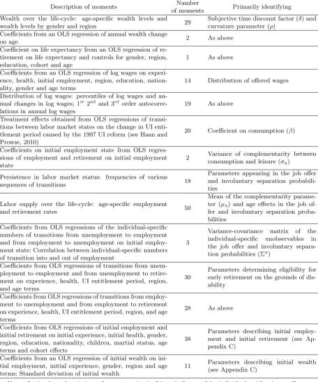
Figure 1 shows the shares of employment, unemployment and retirement by age for men and women and for east and west Germans, averaged over the observation period. We note that early retirement common for individuals in their late 50s and early 60s. Further, there are large differences in employment and retirement behavior according to region of residence: averaged over the whole age distribution, the employment rate is about 10 percentage points higher in west Germany than in the east, and older east Germans have a higher propensity to
15We assume that family composition does not change in the future. However, our model is fully applicable to
individuals who have experienced alternative household compositions, specifically martial status and dependent children, before entering the sample. Appendix C explains how this is achieved.
16Our definition of retirement corresponds closely to observed behavior: Fewer than 5% of retired individuals
are simultaneously in employment and only 1% of retired individuals report that they work full-time. Fewer than 1% of the sampled individuals continue to work beyond age 65 years.
17Given our sample selection criteria, less than 5% of the male (female) population under study works fewer
Figure 1: Employment, unemployment and retirement over the life-cycle by gender and region of residence (a) Women 0 .2 .4 .6 .8 1 Proportion
40 45 50 55 60 65
Age (years)
Full−time employment Unemployment Retirement (b) Men 0 .2 .4 .6 .8 1 Proportion
40 45 50 55 60 65
Age (years)
Full−time employment Unemployment Retirement
(c) West Germany
0 .2 .4 .6 .8 1 Proportion
40 45 50 55 60 65
Age (years)
Full−time employment Unemployment Retirement
(d) East Germany
0 .2 .4 .6 .8 1 Proportion
40 45 50 55 60 65
Age (years)
Full−time employment Unemployment Retirement
retire than west Germans of the same age. These differences are likely related to the relatively poor economic conditions in east Germany.
The SOEP data set includes individuals’ gross earnings in the month prior to the interview date. Using the corresponding working hours, including hours of payed overtime work, we construct a gross hourly wage measure. We follow Fuchs-Schuendeln and Schuendeln (2005) and construct a measure of individual-level wealth based on the yearly financial information available in the SOEP. Specifically, an individual’s wealth is defined as the sum of net property equity and non-property wealth, where the latter is computed from capital income assuming a real rate of return of 3% per annum.18 Wealth and wages are converted to year 2000 prices using the Retail Price Index. The average observed gross hourly wage is 15.65 Euros and average individual wealth is 40037 Euros.
3.2 Human Mortality Database (HMD)
We obtain information about longevity in Germany from the relevant life tables in the Human Mortality Database (HMD).19The life tables include survival probabilities and life expectancies that vary by age, birth cohort, region of residence (east or west Germany) and gender and are available for the years 1991 - 2007. Based on the information in the HMD, we assign a
18A real interest rate of 3% per annum is in line with the rates prevailing in the capital markets: Deutsche
Bundesbank (2001) reports an average ex ante real interest rate of 3.13% in Germany for the period 1994-2001 (based on estimated inflation), and this result is supported by the calculations of Garnier et al. (2005).
19Human Mortality Database is provided by the University of California, Berkeley (USA) and Max Planck
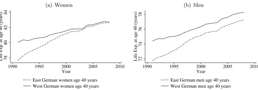
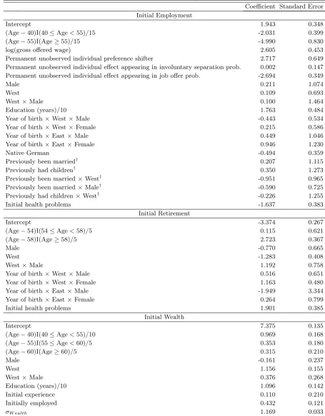
Figure 2: Life expectancy at age 40 years: evolution over time in east and west Germany
(a) Women
78
80
82
84
Life Exp. at age 40 (years)
1990 1995 2000 2005 2010
Year
East German women age 40 years West German women age 40 years
(b) Men
72
74
76
78
Life Exp. at age 40 (years)
1990 1995 2000 2005 2010
Year
East German men age 40 years West German men age 40 years
Source: Authors’ calculations based on the Human Mortality Database.
demographic group-specific and cohort-specific survival probability and life expectancy to each observation in our SOEP sample.20
Figure 2 shows the evolution over time of life expectancy at age 40 years for east and west German men and women. As expected, we observe longer life expectancies for women and, irrespective of gender or region, an upward trend in life expectancy over time. As well documented in the demographic literature, e.g., Gjon¸ca et al. (2000), life expectancy in east Germany in 1991, immediately after German reunification, was considerably lower than in west Germany: in 1991 a 40 year old east German man expected to live 2.7 years less than his west German counterpart, and the corresponding difference for women was 2.4 years. More important for our purposes are the different time trends by gender and region: between 1991 and 2007, there was a strong east-west convergence in life expectancy for women and moderate east-west convergence for men. Specifically, by 2003 there was hardly any east-west difference in life expectancy for women and by 2007 the east-west life expectancy gap for men had fallen to one year. According to Gjon¸ca et al. (2000), Nolte et al. (2002) and Kibele and Scholz (2008), the leading reason for this convergence was improvements in the medical system in east Germany.
In light of the above documented heterogeneity in life expectancy, in the empirical implemen-tation of our structural life-cycle model we permit variation in life expectancy according to age, birth cohort, gender and region of residence. This maximizes the model’s accuracy. Further-more, by drawing on variation between demographic groups in the extent of improvements in life expectancy over time, we are able to estimate the relationship between life expectancy and retire-ment decisions, controlling for age, time and cohort effects. This quantity is informative about the extent to which individuals condition behavior on objectively-measured life expectancy. As a powerful in-sample goodness of fit test, we compare the relationship between life expectancy and retirement decisions as implied by our estimation results with the corresponding quantity
20The HMD does not contain information about marital status. In general, the life expectancy of single
observed in our sample.21
4
Estimation Strategy and Results
4.1 Estimation, Identification and Treatment of the Initial Conditions
As in Gourinchas and Parker (2002), French (2005) and French and Jones (2011), we estimate the parameters of our model using the Method of Simulated Moments (MSM): parameters are chosen to minimize the distance between a set of moments pertaining to the values of the endogenous variables, namely wages, wealth levels, and employment and retirement outcomes, as observed in our sample and the average values of the same moments in a number of simulated data sets. The construction of each simulated data set starts from the empirical distribution of the exogenous individual characteristics, such as gender, education and region of residence, observed in our sample. Given a trial parameter vector θt, we simulate initial values of the endogeneous variables by drawing from a reduced form model. We then simulating wage offers and employment, retirement and consumption outcomes in subsequent quarters of the sample period based on the above-described structural model. The value function is approximated using the simulations and interpolation method described in Appendix A.
Suppose that a total of p moments are used in the MSM estimation. Let Mo denote the p-by-1-dimensional vector of moments constructed from our sample observations. Further, let Ms
k(θt) denote the same vector of moments constructed using thek
th simulated sample obtained
using the parameter vectorθt. The MSM parameter estimates are the value ofθtthat minimizes the weighted quadratic distance (Ms(θt)−Mo)′W(Ms(θt)−Mo), where W is a fixed p-by-p-dimensional positive semidefinite weighting matrix and Ms(θt) denotes the value of the vector of simulated moments averaged over K simulated data sets, each obtained using the parameter vector θt.22 Under the conditions stated in Pakes and Pollard (1989), the MSM estimator is consistent and asymptotically normally distributed.
Estimation uses 265 moments and we estimate 82 parameters. The subjective time discount factor, δ, and the utility curvature parameter, ρ, are identified from information on wealth holdings and saving behavior according to age; knowledge of average wealth is sufficient to identify either δ orρ, while with additional information on variation in wealth according to age we can identify both parameters. Ordinary Least Squared (OLS) coefficients from regressions of wages and transitions between labor market states on demographic variables provide moments that identify the effects of observed individual characteristics on wages, job offers and involuntary separations. See Appendix B for further details.
As described in Section 3.1, we sample wages only in quarters that coincide with the ad-ministration of the annual SOEP survey and only for employed individuals who answered all
21In different settings, Alesina and Fuchs-Schuendeln (2007), Fuchs-Schuendeln (2008) and Fuchs-Schuendeln
and Schuendeln (2005) also exploit variation generated by German reunification.
required survey questions. Our estimation strategy accounts for selectivity in wage observations. We therefore represent correctly the financial incentive to work and capture accurately the value of future public pension benefits. In the MSM estimation routine we account to selectivity in wages by matching moments based on sample wage observations with moments constructed us-ing simulated wage draws that have survived the same selection mechanisms as the sample wage observations.23 A simulated wage draw is included in the construction of the simulated moments if and only if: (i) employment is the individual’s optimal choice in the simulated sample; (ii) the quarter is one in which the individual was surveyed; and (iii) the observation survived random elimination of accepted wage draws designed to account for non-random non-response.24 Non-labor income and non-linearities in the tax and transfer schedules provide exclusion restrictions and thus ensure that identification of the parameters in the wage equation is not reliant purely on functional form.
Appendix C provides further details concerning our treatment of the initial conditions and presents estimates of the parameters that characterize the initial conditions. We note here that the parameters appearing in the initial conditions are estimated jointly with the structural parameters. Further, by including unobservables that may affect both the initial conditions and subsequent behavior, our estimation methodology accounts fully for the endogeneity of the initial observations of individuals’ experience, wages, wealth and employment status.25
4.2 Goodness of Fit and Structural Parameter Estimates
The estimated model is able to fit the observed relationship between life expectancy and re-tirement. We thus conclude that our model provides a sound basis for counterfactual policy simulations which investigate the effect of life expectancy on life-cycle behavior. In more de-tail, we obtain a summary measure of the observed relationship between life expectancy and retirement by running an OLS regression of retirement on age 65 life expectancy, age dummies, cohort dummies and time dummies. (We are able to separate cohort effects from the effect of life expectancy due to the presence of differences between demographic groups in the extent of improvements in life expectancy over time.) The coefficient on life expectancy in this OLS regres-sion is -0.066 (with a robust individual-level clustered standard error of 0.027). Meanwhile, the corresponding coefficient on life expectancy implied by the estimated structural model is -0.059, which is less than 0.3 of a standard error away from the corresponding observed quantity.
Our model is also able to replicate observed features of: the distributions of wages and changes in wages; life-cycle labor supply and retirement behavior; the age profile of wealth; and the patterns of transitions between employment and unemployment (see Appendix D).
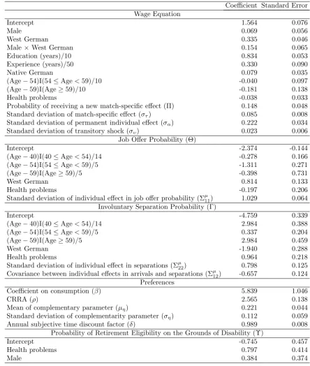
Table 1 reports the structural parameter estimates. Looking first at the wage equation, we
23Note that our structural model features the joint determination of wage and employment outcomes and
therefore accepted simulated wage offers are subject to the same selectivity as sample wage observations. 24We estimate the probability of an employed individual refusing to answer one or more of the survey questions
required to construct the hourly wage. We then exclude the simulated wage draws of employed individuals with the same probability. This method assumes that survey non-response is base purely on observables.
25Health, measured by an indicator of the individual having health problems that limit daily activities, enters
Table 1: Structural parameter estimates
Coefficient Standard Error Wage Equation
Intercept 1.564 0.076
Male 0.069 0.056
West German 0.335 0.046
Male×West German 0.154 0.065
Education (years)/10 0.834 0.053
Experience (years)/50 0.330 0.090
Native German 0.079 0.035
(Age−54)I(54≤Age<59)/10 -0.040 0.097
(Age−59)I(Age≥59)/10 -0.181 0.138
Health problems -0.038 0.033
Probability of receiving a new match-specific effect (Π) 0.148 0.048
Standard deviation of match-specific effect (στ) 0.085 0.008
Standard deviation of permanent individual effect (σα) 0.222 0.034
Standard deviation of transitory shock (συ) 0.023 0.006
Job Offer Probability (Θ)
Intercept -2.374 -0.144
(Age−40)I(40≤Age<54)/14 -0.278 0.166
(Age−54)I(54≤Age<59)/5 -1.311 0.271
(Age−59)I(Age≥59)/5 -0.398 0.731
West German 0.814 0.133
Health problems -0.197 0.206
Standard deviation of individual effect in job offer probability (Σµ11) 1.029 0.064 Involuntary Separation Probability (Γ)
Intercept -4.759 0.339
(Age−40)I(40≤Age<54)/14 2.984 0.388
(Age−54)I(54≤Age<59)/5 0.337 0.204
(Age−59)I(Age≥59)/5 2.984 0.459
West German -1.940 0.288
Health problems 0.964 0.218
Standard deviation of individual effect in separations (Σµ22) 0.798 0.125 Covariance between individual effects in arrivals and separations (Σµ12) -0.657 0.124
Preferences
Coefficient on consumption (β) 5.839 1.046
CRRA (ρ) 2.565 0.138
Mean of complementary parameter (µη) 0.221 0.044
Standard deviation of complementarity parameter (ση) 0.112 0.059
Annual subjective time discount factor (δ) 0.989 0.008
Probability of Retirement Eligibility on the Grounds of Disability (Υ)
Intercept -0.745 0.457
Health problems 0.797 0.414
Male 0.384 0.374
Notes: “Health problems” is an indicator of the individual having health problems that limit daily activities. The mean and standard deviation of the complementarity parameter (ηi) after allowing for truncation are 0.231 (with a standard error of 0.023) and 0.106 (with a standard error of 0.028) respectively.
is 8.34%. Unobservables are found to play an important role in wage determination. Of the permitted unobservables, the permanent individual effect (αi) has the highest standard devia-tion and therefore has the largest impact on wage offers. This finding implies that unobserved differences in wages are driven primarily by differences in permanent unobserved individual char-acteristics. However, we also find a significant unobserved match-specific effect; quantitatively, we find that each quarter an individual has a 14.8% chance of receiving a new match-specific draw. This corresponds to an individual receiving a new match-specific draw on average every 6.8 quarters.26
The job offer and involuntary separation probabilities display clear age patterns: older indi-viduals are less likely to receive a job offer and are more likely to be subject to an involuntary separation than younger individuals. As expected, those in poor health and those living in east Germany are relatively likely to experience an involuntary separation and are relatively unlikely to receive a job offer. Unobserved individual characteristics have significant effects on the job offer and involuntary separation probabilities. The unobservables affecting job offers and invol-untary separations are significantly negatively correlated, a result which is consistent with those unobserved characteristics that contribute positively to involuntary separations also having a negative effect on the probability of receiving a job offer. We find that the probability of being eligible for early retirement on the grounds of disability is positively and significantly (at the 5.4% level) related to the presence of health problems.
The coefficient on consumption,β, is significantly greater than zero which implies that indi-viduals’ behavior is influenced by the financial incentives associated with employment, retirement and wealth accumulation. We find that ηi, the individual-specific parameter that describes the complementarily between consumption and leisure, varies significantly over individuals. More-over, after allowing for truncation of ηi from above at 0.999 and from below at 0, the mean value of ηi is 0.231. This implies that on average 23.1% of consumption is required to com-pensate an employed individual for the disutility of working. Our estimate of the annualized subjective time discount factor is 0.989, a figure which is in line with previous findings (e.g., De Nardi et al., 2010). Finally, our estimate the CRRA parameter, ρ, is 2.565 and we therefore individuals are risk averse. Both the subjective time discount factor and the CRRA parame-ter are precisely estimated, which lays testament to the quality and relevance of the available consumption information.
5
Policy Analysis
5.1 Longevity, Life-cycle Behavior and Government Revenue
The behavioral and fiscal implications of increasing life expectancy must be understood prior to determining how public pension systems may be reformed to ensure financial stability in the face of improving longevity. We thus commence our counterfactual analysis by using our estimated structural life-cycle model to explore the effects of an increase in life expectancy. Specifically, we compare the optimal life-cycle behavior, and associated tax, transfer and pension receipts, of
26This results suggests that match-specific wage shocks occur at a higher frequency than job changes. Therefore,
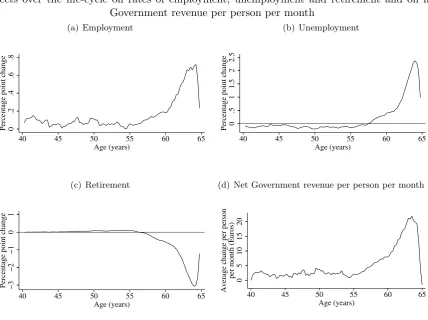
Figure 3: Life expectancy improvement between 1942 and 1982 birth cohorts:
Effects over the life-cycle on rates of employment, unemployment and retirement and on net Government revenue per person per month
(a) Employment
0
.2
.4
.6
.8
Percentage point change
40 45 50 55 60 65
Age (years)
(b) Unemployment
0
.5
1
1.5
2
2.5
Percentage point change
40 45 50 55 60 65
Age (years)
(c) Retirement
−3
−2
−1
0
1
Percentage point change
40 45 50 55 60 65
Age (years)
(d) Net Government revenue per person per month
0
5
10
15
20
Average change per person
per month (Euros)
40 45 50 55 60 65
Age (years)
Notes: All figures refer to individuals aged 40-64.75 years.
two groups of individuals who differ only with respect to life expectancy. Each individual in the first group is assigned the appropriate gender-specific and region-specific life expectancy of the 1942 birth cohort, that is the life expectancy of an individual from the appropriate demographic group who was 65 years old in 2007. Meanwhile, each individual in the second group is assigned the appropriate predicted individual-specific life expectancy of the 1982 birth cohort, who will reach age 65 years 40 years after individuals in the first group, i.e., in 2047. According to the HMD for Germany, life expectancy at age 65 is anticipated to be on average 6.4 years higher for the 1982 birth cohort than for the 1942 birth cohort.27 For both groups of individuals, we fix the distribution of all characteristics other than life expectancy at that observed in our sample and we impose the year 2007 tax, transfer and pension systems throughout.
Figures 3(a) - 3(c) show how the rates of employment, unemployment and retirement are affected by the 6.4 year increase in age 65 years life expectancy anticipated to occur over the next 40 years. This increase in life expectancy reduces the retirement rate by an average of approximately 1 percentage point for those aged 57-64.75 years and by almost 3 percentage points for individuals aged 64 years. The postponement of retirement among individuals approaching the full pensionable age of 65 years is balanced by an increase in unemployment and, to a
27The corresponding increase in life expectancy at birth over the 40 years that separate these two cohorts is
Table 2: Life expectancy improvement between 1942 and 1982 birth cohorts:
Effects on average net Government revenue per person, years of employment post age 40 years, retirement age and weighted pension points upon retirement.
Birth Public Pension: Average Life Net Government Revenue Per Person Yr Emp.
Ret. Age Pension
Cohort FPA/ Pension Value Exp. at 65 All Emp. Unemp. Retired Age≥40 Points
1942 65/ 2007 System 83.3 57005 288249 -30682 -200562 17.75 62.35 39.29
1982 65/ 2007 System 89.7 -18446 294666 -31995 -281117 17.78 62.43 39.34
Change (1982−1942 cohort) 6.4 -75451 6418 -1312 -80556 0.03 0.08 0.05
Notes: “FPA” refers to the full pensionable age and “Pension Value” is the per-year value of public pension benefits. “Net Government Revenue Per Person” is the average per person (starting at age 40 years and continuing until death) net revenue received by the Government, measured in Euors. “Yr Emp. Age≥40” is the average number of years of employment post age 40 years and “Ret. Age” is the average age of retirement. “Pension Points” is the average number of weighted pension points accumulated prior to the date of retirement.
lesser extent, an increase in employment. There are two factors which lead the postponement of retirement to be balanced predominantly by higher unemployment. First, those wanting to retire later may have difficulty finding a job due to the relatively low rate of job offers and the relatively high rate of involuntary separations experienced by older individuals. Second, the long entitlement period for Unemployment Insurance provide strong incentive for individuals to use unemployment as a stepping-stone into retirement (see Appendix E.2).
Next, we consider the effect of an increase in life expectancy on net Government revenue, NGR, which takes the following form
NGR = Income Tax + 2×SSC−UIB−SAB−Public Pension Benefits, (16)
where Income Tax consists of taxes paid on labor income, pension income and interest income from wealth holdings, SSC denotes individual Social Security Contributions (this figure is multi-plied by two because firms must match individuals’ contributions), and UIB and SAB correspond respectively to Unemployment Insurance benefits and Social Assistance benefits. Figure 3(d) shows that the increase in public pension demands associated with longer life expectancy is offset partly by higher revenue receipts from individuals aged below the full pensionable age. Net Government revenue per person increases at every age prior to the full pensionable age of 65 years. Reflecting the age profile of responses in labor supply and retirement, we find the largest increase in net Government revenue for individuals aged 64 years.
Table 3: Life expectancy improvement between 1942 and 1982 birth cohorts: Implications for wealth accumulation and consumption
Birth Public Pension: Wealth on Monthly Income Total Cons. Monthly Consumption Cohort FPA/Pension Value Retirement from Wealth post Age 40 Age 45 Age 55 FPA (Age 65)
1942 65/ 2007 System 27371 146 571197 1291 1341 1054
1982 65/ 2007 System 28402 126 665166 1294 1336 1035
Difference (1982−1942 cohort): 1031 -20 93969 3 -5 -19
Notes: “Wealth on Retirement” is average per-person private wealth at the date of retirement. “Monthly Income from Wealth” is the average per-person actuarially fair monthly annuity income wealth at the date of retirement. Consumption (Cons.) figures are averaged over individuals. Consumption and wealth figures are in Euros. “FPA” refers to the full pensionable age.
increase by 80556 Euros per person.
Last, we analyze the effect of life expectancy on consumption choices and wealth accumula-tion. In response to an increase in life expectancy, optimizing individuals adjust consumption to equalize the higher return to saving with marginal utility of contemporaneous consumption, which in turn depends on current employment behavior. Empirically, Table 3 shows that the considered 6.4 year increase in age 65 life expectancy leads average individual wealth at the date of retirement to increase by 1031 Euros.28 This result, which is in line with the findings of De Nardi et al. (2009) and De Nardi et al. (2010), demonstrates that the ability to alter wealth accumulation decisions provides individuals with a valuable means of adjusting behavior in response to an improvement in longevity. Recognition of this fact is necessary for understand-ing the effects of reductions in the generosity of the public pension system, discussed below in Section 5.2.
Table 3 further shows that the increase in life expectancy anticipated to occur between the 1942 and 1982 birth cohorts leads to a 21 Euros per month fall in the income stream that retired individuals are able to obtain from accumulated wealth. Thus, increased wealth accumulation prior to retirement is insufficient to compensate for the effect of higher life expectancy on the feasible income stream obtainable from wealth holdings. Due to increased pension point accumu-lation prior to retirement, we find that the considered increase in age 65 life expectancy causes average monthly consumption at age 65 years and above to fall by slightly less than the decline in the feasible income stream obtainable from accumulated wealth. Specifically, consumption at age 65 years and above falls by an average of 19 Euros per month.
Notwithstanding the fall in the average monthly consumption of retired individuals, the 6.4 year increase in age 65 years life expectancy anticipated to occur between the 1942 and 1982 birth cohorts causes expected total per-person post age 40 years consumption to increase by approximately 94000 Euros. As shown in Table 2, roughly 75000 Euros of this increase is accounted for by increased transfers from the Government. Meanwhile, the remaining 19000 Euros of this increase is financed from increased wage income and additional interest income from wealth. Indeed, one of the effects of the improvement in longevity under study is to cause the survival rate prior to the full pensionable age of 65 years to increase. Holding fixed employment and retirement choices, this change leads to an increase in expected life-time wage income.
28This effect consists of a component arising from changes in savings decisions and a component due to
5.2 Public Pension Reform
The substantial deterioration in the Government’s budgetary position created by an increase in life expectancy suggests an important role for public pension reforms. With this in mind, we consider the 6.4 year increase in age 65 life expectancy anticipated to occur over the 40 years that separate the 1942 and 1982 birth cohorts and we analyze the behavioral and fiscal effects of: (i) increases in the full pensionable age; and (ii) cuts in the per-year value of public pension benefits. Throughout this analysis, we continue to fix the distribution of all characteristics other than life expectancy at that observed in our sample and we impose the year 2007 tax and transfer systems. Unless otherwise indicated, we use the 2007 public pension system.
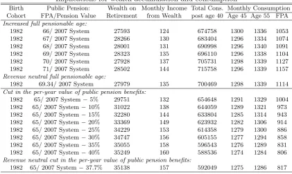
The top panel of Table 4 summarizes the effects on labor market behavior and net Govern-ment revenue of increasing the full pensionable age from its current value of 65 years.29 We find that increases in the full pensionable lead individuals to postpone retirement and to increase years of employment prior to retirement. Within the range of reforms under consideration, a one year increase in the full pensionable age causes the average retirement age to increase by approximately 0.9 of a year, and causes average years of employment prior to retirement to increase by 0.85 of a year. The strong dependence of the employment rate on the age-based eligibility requirements of the public pension system demonstrates that, for many individuals, the rules that control access to public pension benefits are binding constraints on behavior. This finding is entirely consistent with the specifics of the institutional rules. Indeed, according to the 2007 public pension system, for the vast majority of individuals, retirement prior to the full pensionable age either was not possible or was associated with reduced public pension benefits (see Appendix F.3). An increase in the full pensionable age, and the associated age-based eligi-bility requirements, therefore raises the age at which most individuals can receive public pension benefits of a given level of generosity.
In terms of fiscal effects, we find that increases in the full pensionable lead to appreciable increases in the average net transfer made to the Government from employed individuals, and cause substantial reductions in the average transfer payment made to retired individuals. Over-all, our calculations suggest that the full pensionable age must be increased to 69.34 years to offset the fiscal consequences for the Government of 40 years worth of growth in life expectancy. In other words, a 6.4 year increase in age 65 life expectancy requires that the full pensionable age be increased by 4.34 years in order to restore the Government’s budgetary position.30 This policy eliminates the approximately 75000 Euros per-person deficit created by 40 years worth of growth in life expectancy via two main routes. First, an increase of 4.34 years in the full pensionable age increases the net transfer received by the Government from employed individ-uals by an average of approximately 54000 Euros per person. Second, the net transfer made to retired individuals declines by an average of roughly 23000 Euros per person.
The bottom panel of Table 4 summarizes the effects on labor market behavior and net Government revenue of cuts in the per-year value of public pension benefits. Throughout these
29When conducting this analysis the age-based requirements for early retirement were increased in line with
the increase in the full pensionable age.
30This figure was obtained by computing the net Government revenue associated with full pensionable ages of
Table 4: Public pension reforms:
Effects on average net Government revenue per person, years of employment post age 40 years, retirement age and weighted pension points upon retirement
Birth Public Pension: Net Government Revenue Per Person Yr Emp.
Ret. Age Pension
Cohort FPA/Pension Value All Employed Unemployed Retired Age≥40 Points
Increased full pensionable age:
1982 66/ 2007 System -65 308534 -31787 -276812 18.70 63.37 40.31
1982 67/ 2007 System 16392 320443 -32192 -271860 19.52 64.26 41.18
1982 68/ 2007 System 33096 332352 -33240 -266016 20.31 65.24 42.04
1982 69/ 2007 System 48140 341927 -33952 -259835 20.99 66.04 42.76
1982 70/ 2007 System 68620 356808 -33393 -254796 21.99 66.99 43.84
1982 71/ 2007 System 88413 371205 -33269 -249522 22.97 68.00 44.85
Revenue neutral full pensionable age:
1982 69.34/ 2007 System 57005 348609 -33314 -258290 21.42 66.39 43.24
Cut in the per-year value of public pension benefits:
1982 65/ 2007 System−5% -6198 295143 -32936 -268405 17.79 62.58 39.39
1982 65/ 2007 System−10% 5427 295281 -33919 -255936 17.79 62.72 39.41
1982 65/ 2007 System−15% 16242 295205 -35060 -243903 17.77 62.86 39.43
1982 65/ 2007 System−20% 26699 295184 -36275 -232211 17.75 63.02 39.45
1982 65/ 2007 System−25% 36448 294996 -37609 -220938 17.72 63.19 39.47
1982 65/ 2007 System−30% 45290 294589 -38998 -210301 17.70 63.36 39.48
1982 65/ 2007 System−35% 53135 294053 -40520 -200398 17.66 63.54 39.48
1982 65/ 2007 System−40% 60231 293466 -41806 -191429 17.62 63.69 39.47
Revenue neutral cut in the per-year value of public pension benefits:
1982 65/ 2007 System−37.7% 57005 293666 -41205 -195456 17.63 63.62 39.47
Notes: See Table 2.
calculations the full pensionable age is held fixed at its current value of 65 years. This set of reforms has little effect on employment outcomes. Further, cuts in the per year value of public pension benefits have only a minor postponement effect on retirement: we find that the average age of retirement increases by 0.20 of a year for every 5 percentage point cut in the per-year value of public pension benefits. These behavior adjustments reflect partly that high wage individuals are most affected by a cut in the per-year value of public pension benefits. Such individuals are likely to be employment, and hence are generally unable to increase employment. Furthermore, a cut in the per-year value of public pension benefits has an ambiguous effect on employment and retirement incentives: A cut in the per-year value of public pension benefits reduces expected income in retirement for while simultaneously cutting future returns to current employment -the associated income and substitution effects work in opposite directions. Thus, even when affected individuals are in a position to adjust behavior, the realized behavior response may be small, as is the case here. Cuts in the per-year value of public pension benefits cause net Government revenue to increase due to considerably lower net transfers to retired individuals. We find that the per-period value of public pension benefits must be reduced by 37.7% in order to counterbalance the fiscal consequences of 40 years worth of growth in life expectancy.
We conclude our analysis of public pension reforms with Table 5, which explores the effects of increases in the full pensionable age and cuts in the per-year value of public pension benefits on individuals’ wealth accumulation and consumption behavior. Mirroring the different responses of labor supply and retirement, we find that the two reforms have distinctly different implications for wealth accumulation and consumption behavior.