The Multiple Discrete Continuous Extreme Value Model (MDCEV) with fixed costs

(1)

Munich Personal RePEc Archive

The Multiple Discrete-Continuous

Extreme Value Model (MDCEV) with

fixed costs

Tanner, Reto and Bolduc, Denis

Université Laval, Département d’Économique

23 July 2012

Online at

https://mpra.ub.uni-muenchen.de/41452/

(2)

The Multiple Discrete-Continuous Extreme Value Model (MDCEV) with fixed costs July 2012

The Multiple Discrete-Continuous Extreme Value Model

(MDCEV) with fixed costs

Abstract

In this paper, we present a model that can be viewed as an extension of the traditional Tobit model. As

opposed to that specific model, ours also accounts for the the fixed costs of car ownership. That extension is

needed since being carless is an option for many households in societies that have a good system of public

transportation, the main reason being that carless households wish to save the fixed costs of car ownership.

So far, no existing model can adequately map the impact of these fixed costs on car ownership. The Multiple

Discrete-Continuous Extreme Value Model (MDCEV) with fixed costs fills this gap. In fact, this model can

evaluate the effect of policies intended to influence household behaviour with respect to car ownership,

which can be of great interest to policy makers. Our model makes it possible to compute the effect of

policies such as taxes on fuel or on car ownership on both the share of carless households and the average

driving distance.

We calibrated the model using data on Swiss private households in order to be able to forecast responses to

policies. One result of particular interest that cannot be produced by other models is the evaluation of the

impact of a tax on car ownership. Our results show that a tax on car ownership has a much lower impact on

aggregate driving demand – per unit of tax revenues – than a tax on fuel.

(3)

Introduction

Being carless is an option for many households in economies having good system of public transportation –

as it is the case in Switzerland. Thus, a good model should be able to map this option. In particular, it should

also be able to map how the fixed costs of holding a car affects car ownership. So far, no model can be found

in the literature that adequately maps this option. This paper presents the theoretical model that fills this gap.

The drawbacks of the existing modelling techniques can be summarized as follows: The OLS fails to map

carless households. The Tobit model is unable to map the impact of fixed costs. The sample selection model

fails due to the lack of an instrumental variable: there is no variable that influences only the choice of

whether or not to own a car whilst not influencing the demand for driving at the same time. An interesting

candidate for solving this problem is the Discrete-Continuous Choice model introduced by Dubin and

McFadden (1984). This model can be used to explore the ownership of certain car types and their use.

Unfortunately, the model only allows the choice of being carless to be captured if the annual mileage

travelled using public transport is given in the dataset. Since this information is not available in most

micro-census datasets, this model cannot be applied.

The Multiple Discrete-Continuous Extreme Value Model (MDCEV) with fixed costs overcomes the

drawbacks of these models. As mentioned above, the proposed model can measure the impact of changes in

the fixed costs of cars on driving demand and on the probability of households being carless. This ability to

map the impact of income, fuel price and the fixed costs of car ownership on both car ownership and car use

could not be found in the literature.1_{The MDCEV model makes it possible to compute the effects of policies}

such as taxes on fuel or car ownership on both the share of carless households and the average driving

distance.

The MDCEV model was introduced by Bhat (2005).2_{This model consists of a direct utility function and a}

budget restriction. It is assumed that it maps the utility maximisation process of a household and is based on

1 One exception is the model of De Jong (1990), used later by Ramjerdi and Rand (1992) and Bjorner (1999). In contrast to our model, it is based on an indirect utility function instead of a direct function. Unfortunately, De Jong's (1990) model has an assumption that violates its compatibility with a microeconomic utility maximisation framework. In addition, it yields rather unrealistic results, particularly with respect to the impact of changes in fixed costs on car ownership. We believe that the MDCEV model with fixed costs maps reality much more effectively and lead to realistic results.

2 The first application of Bhat's model was to explain the time tourists spend for different activities. The model reflects that each activity can be chosen or not and how many hours are spent for the activities, subject to the time restriction of 24 hours a day, Bhat (2005). Later, Bhat applied this modeling framework to the case where households can choose to own none, one or several cars of different car types and decide of the driving distances the different cars are used for, Bhat (2006). In this model, Bhat ignores the fact that holding cars causes fixed costs and thus according to the model it would not be irrational to hold a number of cars even when the preference for car driving is low. Thus, we want to overcome this drawback by introducing fixed cost in our MDCEV model.

(4)

the assumption that a household chooses certain amounts of goods from a set of goods including the

possibility of a household choosing not to consume any good at all. This means that a household may choose

not to consume any goods at all. In order to adapt the model for examining car ownership and car use, we

modified this model in two ways: first, we restricted it to the case with only two goods. This means that

households may only choose whether or not to own and use a car and spend the remaining income for a

consumption basket containing any other good. Secondly, we extended this model to the case where driving

a car requires car ownership, incurring fixed costs, which is our contribution to the theory.

Assumption on household behaviour

The basic idea behind the model is described in the following. We assume that all decisions are taken at the

household level. In the case of non-single households, we do not make any assumptions on who might have

the most influence on the driving decisions. We also assume that each household compares the utility yielded

from the following two options: first, it establishes the utility level it would gain if it owned a car. In this

case, the household income would be reduced by the fixed costs of car ownership. Given that the household

would then decide what annual distance x2 it would drive in order to yield maximal utility. Note that the

household spends its remaining income entirely on good one x1, which we consider to be a consumer basket

containing all goods apart from car driving, e.g. housing, food, medical care, holidays, and so on. We assume

that utility is driven exclusively by the kilometres driven and not by the car ownership. Second, we assume

that the household establishes the utility in the case that it decides not to own a car. In this case, it would save

the fixed costs of car ownership and would spend all its income on good one x1. The household then decides

which option would give it the highest utility. This behaviour can be mapped using a standard

microeconomic utility maximisation approach where the utility level can be computed by the direct utility

function. The calculation of households' utility maximisation as described above can be illustrated as

follows:

(5)

1

x

2

x

2 2 −

y k p

2 1 −

y k

p ₁

y p 0

(

1, 2

)

= S2

u x x u

(

x x1, 2

)

S₂

∗

(

x1,x2

)

S₁

∗ ( 1, 2) S1

[image:5.595.70.302.105.308.2]

u x x =u

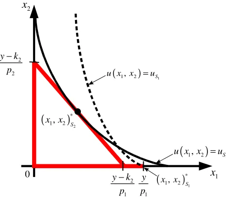
Figure 1: Optimum decisions of two households with different preferences

This figure illustrates the optimal consumption plan of two households with identical income but different

car driving preferences. The solid lined iso-utility curve u x x

(

₁, ₂

)

=u_S₂ represents a household with a high preference for car driving. It decides to own a car – this choice is denoted by index S₂ – and chooses x_2,S₂

∗ _as

its optimal annual driving distance given its income y, the fixed costs of car ownership k₂ and marginal driving costs p₂. We set the price of good one p1 as numeraire, so the utility of x1 can also be interpreted as

the utility of income remaining after having paid all expenses incurred by the car. With this household, the

consumption vector

(

) (

)

1

1, 2 S 1,0

x x ∗ = y p is below the iso-utility curve and therefore yields a lower utility. In contrast, the dashed lined iso-utility curve u x x

(

1, 2

)

=uS₁ represents the household with a low preference

for car driving. Since any point on the budget line defined by points

(

0,

(

y−k2

)

p2

)

and

(

y−k2

)

p1, 0

)

yield a lower utility than spending the total income on good one

(

) (

)

1

1, 2 S 1,0

x x ∗ = y p , the household decides

not to own a car. This choice is denoted by index S₁.

(6)

Derivation of the MDCEV Model and its Maximum Likelihood function

Our choice of the utility function corresponds to the one in Bhat (2005:686). Since in our model, a household

can only choose between the good “annual car driving distance” x2 and consumption basket x1 containing

all other goods, the utility function is then written as:

(

)

1

(

) (

)

2

1 1 exp 2 2

d d

U = X +a + m+ ⋅ ⋅β ς X +a , (1)3

with m= ⋅γ s, (2)

where ς is a logistically distributed stochastic parameter

( )

1

.

1 x

F x

e ς

ς = ₋

+

∼ (3)

We assume a positive marginal utility that is decreasing in all arguments. Thus d1 and d2 are bounded to lie

between zero and one:4 ₀< <_1, =_1,2

j

d j . The smaller dj is, the faster the marginal utility of good j

decreases when Xj increases. Parameters a1 and a2 can be considered as shifting parameters, since they

can move the indifference curves of the utility function along the x- and in the y-axis, respectively. Note that

the marginal utility of X1 is infinite if X1 approaches −a1, which is also true if X2 approaches −a2. The

values −a1 and −a2 therefore define the lower limits of optimal solutions for X1 and X2 respectively. Since

consumption basket X₁ contains essential goods such as food and housing, it must always be consumed. Therefore, a1 is non-positive in order to ensure that the solution for X1 is always positive. Following

Bhat (2008)5_{, we choose} 1=0

a .6_Expression _exp

(

_m+ ⋅β ς

)

_{is a weight on}

(

)

2 2 2

d

X +a . The higher

(

)

exp m+ ⋅β ς is, the stronger is the preference for driving. This weight is determined by socio-demographic

variables in s that influence the preference for driving, m= ⋅γ s. This means, for instance, that households in

rural areas usually have a greater preference for driving than households in urban areas. If a household

3 This utility function is based on the utility function proposed by Bhat (2005:686):

( ) ( )

exp di,

i i i i

i

U=

∑

m + ⋅β ξ ⋅ X +a

where the random terms are assumed to be iid Gumbel distributed: ξj∼iid gu( )0,1 , ( ) exp

( )

x x

f_ξ x =e− ⋅ −e− .

Transforming the utility function by multiplying by exp(m_i+ ⋅β ξ_i)−1 yields Equation (1). Note that the stochastic component ς in (1) corresponds to ς ξ ξ= 2− 1 and is therefore logistically distributed (for a proof see Appendix A1). Note that we use capital letters for X1 and X2, because these variables are also stochastic since their solution in optimality will depend on the stochastic parameter ς .

4 This is to ensure decreasing marginal utility in both goods and the concavity of the utility function, see Appendix A2.

5 “Note that there is no translation parameter γk for the first good, because the first good is always consumed”

Bhat (2008: 290). Note that γk , which Bhat uses, corresponds to αk, which we use.

6 In this case, the so-called INADA-condition ( ) 1

1 2 1

0

lim , ,.., J

x→∂u x x x ∂ = ∞x is fulfilled for x1. It ensures that x1 is greater than zero

when solving the maximisation problem.

(7)

moves from an urban to a rural area, therefore, m is expected to increase in line with an increase in the

household's preference for car driving. The random term ς represents socio-demographic variables sɶ that cannot be observed by the researcher and that can be interpreted as an unobserved preference for car driving.

Following Bhat (2005), we assume this random term to be logistically distributed. Note that the preference

for driving, m, does not contain any car-specific component, since the model captures only one car type,

which is assumed to be the same for each household. To allow for a substantial simplification and to avoid

identification problems, we choose to set: 7

1 2

d =d =d . (4)

We assume that the household maximises its utility by selecting optimal values for X₁ and X₂, subject to its budget constraint:

(

)

1 1 2 2 2 0 2

y= ⋅p X +p ⋅X +I X > ⋅k , (5)

where k2 stands for the fixed costs of car ownership, I X

(

2>0

)

is an indicator function that takes the value

one if X₂>0 and zero otherwise, and the non-negativity constraintX₂≥0.8

The household's utility for the case S₁, where only good one is consumed, is therefore

(

) ( )

1 1 2

1

exp

d

d S

y

u a m a

p

β ς

 

= +  + + ⋅ ⋅

  , with a1=0. (6)

The household's demand for car-km for the case S₂, where the households owns a car, is as follows:

(

)

2 2 1

2 2 1 2 2

2 1

, , , ,

1

y k

A a

p

x y k p p A a

p A

p

−

⋅ −

− =

+ ⋅ and

(

)

1 1 1

2

exp d

p

A m

p β ς

−

 

= ⋅ + ⋅ 

  . (7)

9

7 Bhat (2008) even proposes that some parameter values are fixed: “Alternatively, the analyst can stick with one functional form a priori, but experiment with various fixed values of a_k for the γ_k-profile [...]”; Bhat (2008: 282), footnote 9. The term “functional form” refers to the three utility functions (32) in Bhat (2008: 290). The so-called “γk-profile” corresponds to the model based on the

third utility function of (32) in Bhat (2008: 290). The utility function (1) we use is a positively transformed function of that third utility function; we fix its parameter value d= =d₁ d₂ and estimate all other parameters.

8 Since X₁>0 is ensured by the choice of utility function, condition X₂≥0 does not need to be stated.

9 This Marshallian demand function is obtained by solving the corresponding Lagrangian function. For details, see appendix A3.

(8)

Using this Marshallian demand function, we can now compute the maximum level of utility the household

can achieve:

(

)

2

2 2

2 2 1 1

2 2 2 1 1 1 1 exp 1 1 d d S

y k y k

A a A a

y k p p p

u m a

p p

p p _A _A

p p β ς − −  _⋅ ₋   _⋅ ₋   ₋        = − ⋅ + + ⋅ ⋅ +  _{+ ⋅}   _{+ ⋅}          . (8)

By use of the utility functions (6) and (8), the value of the probability of a household choosing to own a car

can be computed:

(

2 0 | , , , ,1 2 2

)

( )

c

P X = θ p p y k =F_ς ς , (9)

where F x_ς

( )

denotes the density function of the logistic distribution and ςc =ς θc

(

, , , ,p p y k1 2 2

)

corresponds

to the so-called “critical” unobserved preference given all parameters and economic variables at which the

household would switch from owning a car to being carless,

2

−

1

|

ς ς≥c

≥

0

S S

u

and

2

−

1

|

ς ς< c

<

0

S S

u

.10

The density of the Marshallian demand can be computed using the first-order conditions of the Lagrangian

associated with the utility maximisation problem:11

( )

(

)

2 2

1 2 2

1 2 2 1

0

2 2 ₁ ₂

1 1

1 1 1

| , , , , , with 0

X X

V V d p d

f z p p y k s f a

y k p z _a p z a

p ς θ β β ∧ >      ₋  ₋ ₋   − = ⋅ _ _⋅ _{− −} ⋅ + = +     ₊     (10) where

( )

( ) (

)

2 2

1 1

1

ln ln 1 ln y k p z

V d p d

p

 _{− −} 

= − − − ⋅  

 , (10a)

( )

(

) (

)

2=ln −ln 2 − − − ⋅1 ln + 2

V d p m d z a , with

m

= ⋅

γ

s

, and (10b)

( )

(

)

2

1 x x e f x e ς − − = + (10c)

is the density of the logistically distributed random term ς .

10 Note that the Marshallian demand (7) at ςc is always greater than zero and that ςc is always unique. For proof, see

Appendix A5.

11 For details, see Appendix A3.

(9)

Since we assume that the random terms ς are independent across households, the Maximum Likelihood

function is thus:

(

)

(

2 2 1,2,.., | , 1, 2 1,2,.., , 1,2,.., , ,2 1,2,..,

)

MLE n n N n N n N n N

L X =x ₌ θ p p ₌ y ₌ k s₌

(

)

( )

(

)

( )

2 2

0 0

2 1 2 2 0 2 1 2 2

1

0 | , , , , , n | , , , , n ,

N N

I x I x

n n n n X X n n n n

n i n

P x θ p p y k s = f _∧ _> x θ p p y k s >

= =

=

∏

= ⋅

∏

− (11)

where I z

(

>0

)

and I z

(

=0

)

are indicator functions, being one when the argument is true and zero otherwise. Vector

θ

contains all parameters,

θ

=

{

d a

, , ,

₂

γ β

}

. Probability P

( )

i is defined in (9) and density

( )

2 2 0

X X

f _∧ _> i in (10). Index n corresponds to the n-th observation in the dataset.

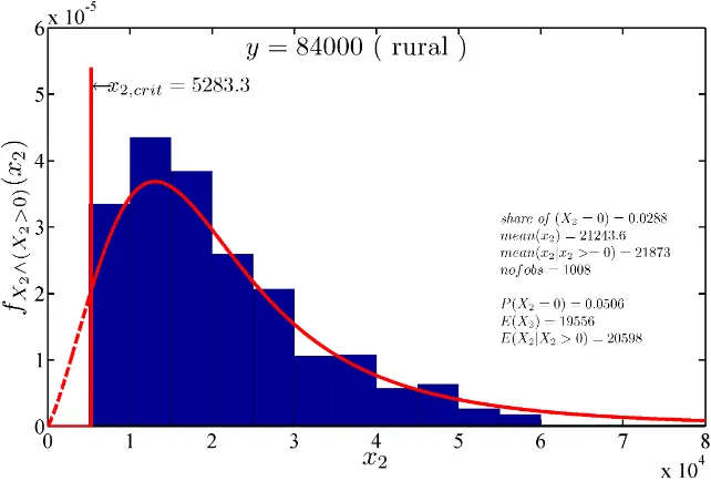
It is important to note that this likelihood function is only defined for values x₂_n =0 and x₂_n≥x₂

( )

ς_{c n}_, , since for values x2n in interval 0<x2n<x2

( )

ςc n, the probability of observation is zero. Thus as soon as any

observation belongs to the interval 0<x2n <x2

( )

ςc n, , the likelihood function (11) equals zero, which makes

it impossible to compute optimal parameters θ using the Maximum Likelihood Estimation routine. We thus

propose an estimation routine where all observations 0<x2n<x2

( )

ςc n, are removed from the dataset before

we apply the Maximum Likelihood Estimation routine. Since the value x₂

( )

ςc n_, only depends on parameters

2

a and d,12_parametersγ _and_β _{can then be computed by Maximum Likelihood estimation using the}

modified dataset and given parameters a₂ and d. Since both a₂ and d also influence the shape of the density function (10) as well as the probability that a household is carless (9), we cannot set them arbitrarily. For this

reason, we propose minimising the following “penalty function” for choosing optimal values for parameters

2

a and d:

( )

(

)

(

)

( )

2 2 ₂

1 2

mean 0 mean # elim. observations

mean 0 mean size of initial observations

sim sim

P X x E X x

Q c c

x x

 ₋ ₌   ₋  _ _

= ₌  + ⋅  + ⋅ 

 

    , (12)

where c₁ and c₂ weigh the corresponding error components and Psim

(

X₂ =0

)

and Esim

( )

X2 are defined as

follows:

(

2

)

(

2 1 2 2

)

1

0 0 | , , , , ,

N

sim n n n n

n

P X P X p p y k s

N = θ

= = ⋅

∑

= , (13)

( )

(

)

( )

2

2 2 2 ,

2 0 1 2 2

1

| , , , ,

n

c n

z y k

N

sim X X n n n n

n _{z x}

E X z f z p p y k s dz

N _ς θ

= −

∧ > = =

= ⋅

∑ ∫

⋅ − . (14)

12 For proof, see Appendix A6.

(10)

Therefore, we propose the following estimation routine:

1. Choose values for d and a₂.

2. Eliminate all observations with 0<x₂n<x₂

( )

ςc n_, from the dataset.

3. Estimate parameters

γ

by MLE conditional on d and a 2 using (11).

4. Compute the penalty function (12).

5. Repeat steps 1 to 4 for a number of different values for d and a₂ (grid search).

6. Choose values d and a2 so that the lowest value of the penalty function is yielded (“optimal values”

d and a2).

Note that functions (13) and (14) are also used to compute aggregate impacts on driving demand and the

probability of being carless when the economic variables p2, k2 and y change, e.g. these functions will be

used to compute the corresponding elasticities.

(11)

Empirical Results

We obtained results using the micro-census data about travel behaviour in Switzerland collected in 2005 by

the Swiss Federal Statistical Office SFSO.13_{We chose this data because it contains a large number of}

observations, namely 33,000, and a number of useful socio-demographic variables concerning the

households. Since our model captures only one car type, it is considered to be an “average car”. The fixed

costs of maintaining a car and the marginal costs of driving are thus assumed to be equal to those of an

average car owned by a Swiss household. The values we retain for k2 and p2 were taken from the Swiss

touring club TCS (2007) and comprise:14 2 7033

k = and p2 =0.1601+0.0778⋅pfuel. (15)

Note that the annual fixed costs k2 mainly consist of depreciation, which is unrelated to the car's use, such as

rusting, and loss in value due to the technical progress of new cars, capital costs, taxes on car ownership and parking costs. Since we neglect such costs as evaluation and registration costs, we assume that owing a car is similar to renting a car and that households can switch from owning a car to being carless without any cost. The costs dependent on the number of kilometres driven consist of fuel costs 0.0778⋅p_fuel and non-fuel-related costs such as the wear of tyres and mechanical components, which account for CHF 0.1601 per kilometre. The fuel price p_fuel is the average fuel price from the last twelve months prior to interviewing the household to which the information on annual driving distance refers.15_{To explain the deterministic}

component of the preference for driving m, we used a dummy “rural” standing for the type of the households' location and a the number of people living in the individual households.

Table 1 below shows the results for two cases. In the case denoted as “∞_{”, expectation value}E_sim

( )

X₂ is computed according to (14); in the case of “60,000 km” the upper limit “

(

yn−k2

)

p2n” is replaced by “

(

)

(

2 2

)

min yn−k p n,60,000km ”. We believe that the latter produces more realistic results since the

theoretical density (10) has some tail above this value, while as the empirical distribution does not, since

households simply have not time to drive such long distances. Thus, integrating to an upper limit above

60,000 km when computing (14) would simply result in too high and therefore unrealistic values.16_Hence,

13 For details see SFSO (2006a) and SFSO (2006b).

14 According to TCS (2007), the total annual costs of an average car amounted to CHF 11,600 when the annual distance driven was 15,000 kilometres (km). 17.4% of these costs, namely CHF 2,018.4, were fuel costs. Based on the average fuel price paid for petrol 98 octane of CHF 1.729/litre in 2007 (SFSO 2009), it can be computed that the TCS (2007) based this fuel cost on a fuel consumption of 7.7825 litres/100 km: (CHF 2,018.4/15,000 km) / (CHF 1.729/litre) = 7.7825 litres/100 km. The fuel costs of an average car per kilometre are therefore 7.7825 litres/100 km/100 multiplied by the fuel price per litre paid by households. Non-fuel-related marginal costs of a car were calculated to be 20.7% of the total costs, 0.207 · CHF 11,600 = CHF 3,312, amounting to CHF 3,312/15,000 km = CHF 0.1601/km, see TCS (2007).

15 The computation of pfuel is based on the monthly average price of petrol 98 octane, as published by the SFSO (2009a).

16 This argument is discussed more in detail in Appendix A7.

(12)

we believe it is justifiable to restrict the upper limit of the integral to this value. For the penalty function (12),

we choose arbitrarily c1=1 and c2=0.5.17 However, it is important to note that changing parameters c1 and

c2 only has a limited impact on the measures of interest, namely elasticities.18 The results processed for the

aforementioned datasets are as follows:

Upper limit of integrating,

E X

( )

₂ ∞ _{60,000 km}

( )2, 2

ε

E X p −₍1.070.0069₎ −(0.670.0075)

( )2, fuel

E X p

ε

(0.490.0031)

−

(0.280.0031)

−

( )2,

ε

E X y (1.170.0031) (0.750.0069)

( )2,2

ε

E X k − 0.16(0.0030) − 0.16(0.0029)

( 2 0 ,) 2

ε

P X₌ p (0.240.0052) (0.240.0049)

( 2 0 ,)

ε

P X = pfuel (0.00005)

0.14

(0.110.0028) ( 2 0 ,)

ε

P X = y −₍1.420.0087₎ −(1.410.0081)

( 2 0 ,) 2

ε

P X = k (1.270.0102) (1.330.0111)

The values in parentheses “(...)” represent standard deviations computed using the bootstrapping method with 10 random samples of 200 obs. each.

Table 1: Simulated elasticities when using a modified density function to compute the expectation value.19

The results yielded by the model for the fuel price elasticities of travelling demand εE X_{( )}₂,pfuel are of major

interest. Since our model assumes no costs when switching from owning a car to being carless and vice

versa, our elasticities can be interpreted as long-term fuel price elasticities. These correspond approximately

to average values determined in international studies (-0.31), such as in Graham and Claister (2004). The

income elasticity of aggregate driving we obtained (0.77) is also very close to the average values established

in international studies (0.73) by both Graham and Claister (2005) and Goodwin et. al. (2004). In contrast,

both values εP X₍ ₂>0 ,₎pfuel =0.026 and εP X( 2>0 ,)y =0.33 that can be computed from εP X( 2=0 ,)pfuel and εP X( 2=0 ,)k2

are quite smaller in absolute value than the elasticities of the car stock determined in international studies.20

We explain this difference by the fact that our elasticities refer to the case of “at least one car” and the

17 Note, that choosing arbitrarily c₁=1 and c₂=0.5 yields that in the optimum the number of “irrational” observations that are removed account for about 9% of the total observations. We propose not to choose values lower than 0.5 for c2, since this would lead to a “dropout-rate” of observations of more than 9%, which we would consider a too high. Note, that removing these observations should not induce a significant change in the elasticities of driving demand we compute, since these households drive a very low annual mileage and thus do not contribute much to the aggregate driving distance.

18 We applied values of 0.5, 1.0 and 2.0 in various combinations on both parameters c1 and c2. Despite this quite dramatic change

in the parameters of the penalty function, the resulting values of _{( )} 2, 2

E X p

ε remained in the region of about 20% of its absolute value, meaning

(

_{( )}

)

(

_{( )}

)

(

_{( )}

)

(

_{( )}

)

2, 2 2, 2 2, 2 2, 2

max ε_{E X} _p −min ε_{E X} _p max ε_{E X} _p +min ε_{E X} _p ⋅0.5 =0.12, while the same measure for _{( )} 2, 2

P X p ε

amounts to 0.2 and for both ₍ ₎ 2 0 ,2

P X p

ε = and εP X( 2=0 ,)y to 0.02.

19 The point estimates are based are based on the complete dataset.

(13)

income elasticity for buying a second or even a third car can be assumed to be greater since the latter can be

considered a luxury good. In contrast, ₍ ₎

2 0 ,2 0.31

P X k

ε > = is quite similar to the values determined by Dargay

(2001) and Johansson and Shipper (1997) for the elasticity of the car stock with respect to the car's fixed

costs.21_{However, it is also important to note that the results found in international studies for the elasticity of}

car ownership vary greatly and thus it is hard to judge whether the values a model yields are plausible.

Furthermore, our model also yields that both elasticities _{( )}

2, fuel

E X p

ε and _{( )}

2 ,

E X y

ε are only weakly driven by

households that switch to being carless, despite them switching from an annual mileage of about 5,000 km to

zero – according to the model.22

Finally, an important result of our model is also that the effect of a tax on car ownership on aggregate driving

distance is – per unit of tax revenue – more than ten times weaker than the effect of a tax on car ownership.23

One criticism of calibrating the model and producing these results by using the micro-census dataset of the

SFSO 2005 is that the fuel price does not vary enough across households. For this reason,we also calibrate

the model by using stated preference datasets with a large variation in fuel price.24_{It is important to note that}

all elasticities with respect to the aggregate driving demand produced by using this dataset differ at most by

13% in absolute terms from the results produced by the micro-census dataset of the SFSO 2005 as presented

in table 1.

20 Note, that ₍ ₎ ( )

( ) ( ) ( ) (( )) ( ) (₍ )₎

2 2

2 2 2 2

0 , 0 ,

2 2 2 2

0 0 0 0

fuel fuel

P X p P X p

fuel fuel

p p

P X P X P X P X

p P X p P X P X P X

ε _> =∂ > ⋅ = −∂ = ⋅ ⋅ = = −ε ₌ ⋅ = =

∂ > ∂ = > >

0.19 1.33 0.31,

81

= − ⋅ = where for P X( ₂=0) we use the value of the dataset from which the observations 0<x₂<X₂( )ςc and

2 60,000 km

x > were removed.

21 The only study in which we could find a model where the effect of a tax on car ownership was examined was in Johansson and Shipper (1997). In their model, this tax was imposed by a tax on car purchase. Annualising one unit of this tax yields an increase in the fixed costs of car ownership of about 2%, yielding a 0.6% decrease in car stock. Thus, a 1% increase in fixed costs would reduce the vehicle stock by 0.3%.

22 This effect contributes only about 2.5% to the total effect on aggregate demand in the case of εE X( )2,pfuel and 11.5% in the case of

( )2,

E X y

ε . ( ) ( ) ( ) ( ) ( ) ( ) ( ) ( ) 2 2 2

2, 0 2

2 2

,

2 2 2 2 2 2 2 2

2 2

0 ,

0 mean 0.28 13,890 km 3889.2 km,

0 0.10 0.1890 5000 94.5km. 94.5 / 3889.2 2.4%.

fuel

P X effect

c E X p

c P X p

dx dP X

dx dx

x x

dp p dp p dp p dp p

P X x

ε ς ε ς = = = = ⋅ = ⋅ = = ⋅ = = = ⋅ = ⋅ = ⋅ ⋅ = = ( ) ( ) ( ) ( ) ( ) ( ) ( ) ( ) 2 2 2

2, 0 2

2 2 2 2 , 2 2 0 , 0 mean 0.80 13,890 km=11,112 km,

0 0.80 0.1890 5000 1275.8 km. 1275.8 /11,112 11.5%.

P X effect

c E X y

c P X y

dx _{dP X}

dx dx

x x

dy y dy y dy y dy y

P X x

ε ς ε ς = = = = ⋅ = ⋅ = ⋅ = = = ⋅ = ⋅ = ⋅ ⋅ = =

23 The relative effect can be computed as follows:

( )2,2 ( )2,2 2

(

mean( )2 mean( 2 0.1601)

)

0.26 0.11 7,033km

(

13,890 km 0( .2745 0.1601)

)

10.5.

E X p E X k k x p

ε ε ⋅ ⋅ − = ≈ ≈ ⋅ ⋅ − =

24 We used the same dataset as Axhausen and Erath (2010). We gratefully thank Prof. Kay Axhausen and Dr. Alexander Erath for providing their dataset.

(14)

Conclusion

In contrast to currently existing models, ours is able to quantify the effects of a tax on fuel and/or a tax on

car ownership on both the car ownership and the cars' use. Our model made it also possible to measure the

effects of two mechanisms leading to a decrease in aggregate driving distance when the fuel price is

increased, namely: The first one is determined by households with a rather high preference for car driving

that will keep the car, but they will reduce their annual mileage. The second mechanism is determined by

households with a rather low preference for car driving will switch form owning a car to become carless and

therefore reducing their annual mileage form about at least 5,000km per year to zero. Our model shows, that

the effect of the first mechanism dominates the one of the second, since only a few households will sell their

car, if fuel prices increase.

Furthermore, the model made it possible to show that a tax on car ownership is – per unit of tax revenue –

much less effective as a tax on fuel. It is noteworthy that the model adapts the data very well, even though

we only estimate four parameters.25

The fact that the model contains a utility function opens the way for more applications such as computing the

Hicksian compensating variation when fuel prices increase for each household or the household's willingness

to pay for car ownership.

25 For details see Appendix A7.

(15)

References

Axhausen, Kay W. and Alexander Erath, 2010, “Long term fuel price elasticity: Effects on mobility tool ownership and residential location choice”, Bundesamt für Energie, 2010, Publikation 29015.

http://www.bfe.admin.ch/php/modules/enet/streamfile.php?file=000000010334.pdf&name=000000290158

Bhat, Chandra R., 2005, “A multiple discrete-continuous extreme value model: formulation and application to discretionary time-use decisions”, Transportation Research Part B 39 (2005), 679-707.

Bhat, Chandra R. and Sudeshna Sen, 2006, “Household vehicle type holdings and usage: an application of the multiple discrete-continuous extreme value (MDCEV) model”, Transportation Research Part B 40 (2006) 35–53.

Bhat, Chandra R., 2008. “The multiple discrete-continuous extreme value (MDCEV) model: role of utility function parameters, identification considerations, and model extensions”, Transportation Research Part B 42 (2008) 274–303.

Bjørner, Thomas Bue, 1999, “Demand for Car Ownership and Car Use in Denmark: A Micro Econometric Model”, International Journal of Transport Economics, Vol. XXVI, No. 3, pp. 377-395.

De Jong, G. C., 1990, “An indirect utility model of car ownership and private car use”, European Economic Review, Elsevier, Vol. 34(5), 971-985, July.

Dubin, Jeffrey A. and Daniel L. McFadden, 1984, “An Econometric Analysis of Residential Electric Appliance Holdings and Consumption”, Econometrica, Vol. 52, No. 2 (Mar., 1984), 345-362.

Goodwin, P and Dargay, J and Hanly, M., 2004, “Elasticities of road traffic and fuel consumption with respect to price and income: a review”, Transport Reviews, 24 (3) , 275-292.

Graham, Daniel and Stephen Glaister, 2001, “Review of income and price elasticities of demand for road traffic”, Final Report. Centre for Transport Studies, Imperial College of Science, Technology and Medicine.

Graham, D.J. and Glaister, S., 2004, “A Review of Road Traffic Demand Elasticity Estimates, Transport Reviews”, 24 (3), 261-276.

Johansson, Olof and Lee Schipper, 1997, “Measuring the Long-Run Fuel Demand of Cars”, Journal of Transport Economics and Policy, September 1997.

Ramjerdi, F. and L. Rand, 1992, “The National Model System for Private Travel”, Institute of Transport Economics. TØI rapport 150/1992. Oslo.

(16)

Swiss Federal Statistical Office SFSO, 2009a, “Konsumentenpreisindex, LIK, Durchschnittspreise für Benzin und Diesel, Monatswerte”, Swiss Federal Statistical Office SFSO, Neuenburg (Switzerland) 2009. http://www.bfs.admin.ch/bfs/portal/de/index/themen/05/02/blank/key/durchschnittspreise.Document.88015.xls

Swiss Federal Statistical Office SFSO, 2006a, “Mikrozensus 2005 zum Verkehrsverhalten”, Swiss Federal Statistical Office SFSO, Neuenburg (Switzerland) 2006.

Swiss Federal Statistical Office SFSO, 2006b, “Mikrozensus 2005 zum Verkehrsverhalten, Kurzversion Fragebogen (Hauptbefragung)”, Swiss Federal Statistical Office SFSO, Neuenburg (Switzerland) 2006. http://www.portal-stat.admin.ch/mz05/files/de/00.xml

Touring Club der Schweiz (TCS), 2007, “Kosten eines Musterautos”. http://www.tcs.ch/main /de/ home/auto_moto/kosten/ kilometer/musterauto.html

(17)

Appendix

A1: The distribution of the random term

ς

of the utility function

As mentioned in footnote 1, the random term is equal to the difference of the two iid gumbel distributed

random variables ξ₁ and ξ₂, ₁, ₂

( )

x exp

( )

x

iid f_ξ x e e

ξ ξ ₌ − _⋅ ₋ −

∼ , _{ς ξ ξ}_{= −}₁ ₂.

The cumulative density function (cdf) of ς can be computed as follows:

First, given that the cumulated density function (cdf) of F_ς

( )

y is equivalent to Fς

( )

y =P X

(

1−X2<y

)

,

thus F_ς

( )

y can then be computed as follows:

( )

(

)

(

)

(

)

( ) ( )

( )

( ) (

)

(

)

(

( )

)

2 1 2 2 1 2

2 1 2 1

2 1 2 2 2

2

2 2

2 1 2 2

1 2 1 2 1 2 1 2

2 1 1 2

1 2

2 2 2 2

1 2 ,

exp exp

x x y x x x y x

x x x x

x x y x x x

x y

x x

x x x x

F y f x x dx dx f x f x dx dx

f x f x dx dx f x F y x dx e

P X X

e e d

y P X y X

x

ς ξ ξ

ξ ξ ξ ξ

=∞ = + =∞ = + =−∞ =−∞ =−∞ =−∞ =∞ = + =∞ =∞ − + − − =−∞ =−∞ =−∞ =−∞ = = = ⋅ = = ⋅ = ⋅ + = ⋅ − ⋅

− < = < +

− =

∫

( )

(

)

(

)

(

( )

)

( )

(

)

2 2 2

2

2 2 2 2 2 2

2 2 2

2

2 2

2

ln 1

2 2 2

ln 1 2

exp exp 1 exp

exp .

y

x x x

e

x y

x x x x y x x

x x x

x

x e

x

e e e dx e e e dx e e e dx

e e dx

− − =∞ =∞ =∞ + − + − − − − − − − =−∞ =−∞ =−∞ =∞ − − + − =−∞ = ⋅ − − = ⋅ − ⋅ + = ⋅ − ⋅ =   = ⋅ −   

∫

This expression can be reformulated by substituting 2 ln

(

1 ,

)

2, 2 ln

(

1

)

y y

q=x − e− + dq=dx x = +q e− + :

( )

ln( 1)

( )

ln( 1)

( )

1

( )

1

exp exp .

1 1

y y

q q q

q e _q e _q _q

y y

q q q

F y e e dq e e e dq f q dq

e e ς ξ − − =∞ =∞ =∞ − − + ₋ − + ₋ ₋ − − =−∞ =−∞ =−∞ = ⋅ − = ⋅ ⋅ − = ⋅ = + +

∫

(18)

A2: Concavity of the utility function

In the following we show that the utility function we use is concave. To do so we show that the Hessian

matrix is negative (semi-)definite. We first compute its diagonal elements:

(

) (

)

2

2 1 exp 0, if and only if 0 1.

j d

j j j j j j j

j

U

d d m X a d

X ξ

−

∂ _{= ⋅} _{− ⋅} ₊ _⋅ ₊ _< _< _<

∂

Since the non-diagonal elements are zero, the Hessian matrix is negative (semi-)definite and therefore the

utility function is concave:

2 2 2

2 2 2 2 2

1 1 2 1

2 2 2

1 2

2 2

1 2 2 2

0

0 and 0

0 j

U U U

X X X X U U U

X X X

U U U

X X X X

∂ ∂ ∂

∂ ∂ ∂ ₌ ∂ ₌ ∂ _⋅ ∂ _> ∂ _<

∂ ∂ ∂

∂ ∂ ∂ ∂

, if and only if 0<dj<1, j=1,2 and

1 1

X > −a and X2> −a2.

The term

2 1 2

U X X

∂

∂ ∂ is equal to zero because the utility function is of the additive separable type.

A3: Derivation of the Marshallian demand function and its probability density function

The derivation of the Marshallian demand function as well as of its probability density function is based on

solving the Lagrangian function representing the case, where the households owns a car.

(

1 1

)

exp

(

) (

2 2

)

(

2 1 1 2 2

)

d d

L= X +a + m+ ⋅ς X +a +λ y− −k p X −p X , with a1=0. (A3.1)

The corresponding first-order conditions are as follows:

(

)

1 1 1 1

1

0

d

d p

X a − λ

⋅ − ⋅ =

+ , (A3.2)

(

)

(

)

1 2 2 2

1

exp _d 0

d m p

X a

ς − λ

⋅ + ⋅ − ⋅ =

+ , with m= ⋅

γ

s. (A3.3)

We first derive the Marshallian demand function. To do so, we solve (A3.2) for λ, insert the result in (A3.3)

and reformulate in order to get the resulting expression:

(19)

1 1

2 2 1

1 1 2

exp 1

d

X a m p

X a d p

ς _ _−

+  + 

=  ⋅ 

+  −   

. (A3.4)

From the budget restriction follows that

(

)

1 2 2 2 1

X = y− −k p ⋅X p . (A3.5)

Including this expression in (A3.4) and solving for X2 yields the Marshallian demand function:

(

)

2

2 1

1

2 2 2 1 2 1 2

2 1

, , , , ,

1

y k

A a A a

p

X x y k p p A a a

p A

p

−

⋅ − + ⋅

= − =

+ ⋅ , (A3.6)

1

with

(

)

1 1 1

2

exp

β ς

−

 

= ⋅ + ⋅ 

 

d

p

A m

p .

Note that

x

2

(

y k

−

2

,

p p

1

,

2

, ,

A a a

1

,

2

)

depends on the random term

ς

and there exists a value

ς ς

=

₀ such

that

(

)

0

2 − 2, 1, 2, , 1, 2 |ς ς≤ ≤0

x y k p p A a a and

x

2

(

y k

−

2

,

p p

1

,

2

, ,

A a a

1

,

2

)

|

ς ς>₀

>

0

. (A3.7)2

Secondly, we derive the probability density function of the Marshallian demand function. To do so, we start

by solving each of the first order conditions (A3.2) and (A3.3) for λ and then taking the logs:

( )

1 ln

V = λ , with: V1=ln

( )

d −ln

( ) (

p1 − − ⋅1 d

) (

ln X1+a1

)

and X1=

(

y− −k2 p2⋅X2

)

p1(A3.8)

( )

2 ln

V + =ς λ , with: V₂=ln

( )

d −ln

( )

p₂ + − − ⋅m

(

1 d

) (

ln X₂+a₂

)

. (A3.9) Plugging (A3.8) in (A3.9) and solving for ς yields:

1 2

V V

ς = − . (A3.10)

From this follows

(

1 2

)

(

1 2

)

P ς < −V V =F V_ς −V . (A3.11)

1 Note that in the case of d1≠d2 the expression resulting when plugging the expression (A3.5) in (A3.4) could not been solved explicitly for X2.

2 For a proof, see Appendix A4.

(20)

We can now compute the density of driving demand at a given driving distance x₂ by deriving (A3.11) with respect to x₂:3

( )

(

)

(

)

2 2

2

1 2 1 2

0

2 1 2

1 1 1 1 | , , , , , X X p d d

f z p p y s f V V

y p z p z a

a p ς

θ

∧ >    ₋ ₋    = − ⋅ ₋ ⋅ + +  ₊      (A3.12)

where V₁ and V₂ are given by (A3.8) and (A3.9),

θ

=

{

d a m, , ,₂

β

}

and f_ς

( )

x is the probability density

function (pdf) of the logistic distribution,

( )

(

)

2

exp 1 exp x x e f x e ς − − = + .

A4: Boundary solution in the case of the model with fixed costs

In this section, we shall show that there exists a so called critical relative preference expressed by parameters

ς

+

m

. If the relative preference is below this level, the demand for car driving yields a boundary solution

that means the driving distance is zero. If the relative preference is above this level, the driving demand will be positive. This means, that – given a fixed value for m – a value

ς ς

= 0 exists such that

(

)

0

2 − 2, 1, 2, , 1, 2 |ς ς≤ ≤0

x y k p p A a a and x2

(

y−k2, p1, p2, A a a, 1, 2

)

|ς ς> 0>0, (A4.1)

where

(

)

2 2 1

2 2 1 2 1 2

2 1 , , , , , 1 − ⋅ − − = + ⋅ y k A a p

x y k p p A a a

p A

p

and

(

)

1 1 1

2

exp β ς −

 = ⋅ + ⋅    d p A m p .

Since this is not obvious when looking only at the utility function and the budget restriction, we prove (A4.1). Note that the value

ς ς

= 0 also plays a role when we show in appendix A5 that ς0 is always smaller

than the critical preference at which the household switch from owning a car to being carless in the case

where owning a car is connected with fixed costs.

3 For this case, the result can also be computed as follows. From P(ς≤ −V₁ V₂)=F V_ς( ₁−V₂) it follows that:

( )( ) ₍( ₎) ( ) ( )

2 2

1 2 1 2 1 2 2

1 2 0

1 2 2

X X

F V V V V V X V

f z f V V

V V z X z z

ς

∧ >

∂ − ∂ − _∂ _∂ _∂ 

= ⋅ = − ⋅ ⋅ − 

∂ − ∂ ∂ ∂ ∂ , where

1 1 1

1 1 1 2

1

0

V X d p

X z x a p

∂ _⋅∂ _{= −} − _⋅− _>

∂ ∂ + , 2 2

1 0

V d

z z a

∂ _{= −} − _<

∂ +

and 2

1 1

y p z

x p

− ⋅

= . Note that the expression 1 2 2 2

V X V

X z z

∂ _⋅∂ ₋∂

∂ ∂ ∂ is positive for any value z that is in the feasible range 0≤ <z y p2. Note that this is a necessary condition for the validity of the theorem of densities of transformed variables.

(21)

The proof that (A4.1) is correct follows from these conditions:

i. lim ₂

(

₂, ₁, ₂, , ₁, ₂

)

0

ς→−∞x y−k p p A a a ≤ ,

ii. lim_ς→∞x2

(

y−k2, p1, p2, ,A a a1, 2

)

>0,

iii. 2

(

2, 1, 2, , 1, 2

)

₀

ς

∂ − _⋅∂ _>

∂ ∂

x y k p p A a a A

A .

Thus, only conditions i., ii. and iii. need to be verified. The proof of condition i. follows from

(

)

1 1 1

2

lim lim exp =0

ς ς β ς

− →−∞ →−∞   =  ⋅ + ⋅    d p A m

p . This implies that

( )

2 2 1 2 2 2 1

lim lim = 0

1

ς→−∞ ς→−∞

−

⋅ −

= − <

+ ⋅ i y k A a p x a p A p .

The proof of condition ii. follows from

(

)

1 1 1

2

lim lim exp =

ς ς β ς

− →∞ →∞   =  ⋅ + ⋅  ∞   d p A m p .

This implies that

( )

2 2

2

1 1

2

2 2 ₂

1 1

lim lim = = 0

1

ς→−∞ ς→−∞

− − ⋅ − ⋅ − = < + ⋅ ⋅ i

y k y k

A a A

y k

p p

x

p p p

A A

p p

.

This result is rather intuitive. If ς → ∞, this means that the household has a very strong preference for car

driving, and it is therefore plausible that it spends all income y−k₂ on car driving.

In order to prove condition iii., the derivative simply has to be computed. This yields:

( )

1

2 2 ₂ ₂ ₂ ₂

2 ₂

1 1

2 1 1 1 1

2 2 1 1 ₁ = = 1 ς ς − _ _ ₋ _ _ _ _ _ _ _ − −   ∂_ ⋅ − ⋅ + ⋅  _ _′_⋅ _{⋅ + ⋅}_ _₋_ _⋅ ₋ __{⋅ ⋅}_′     ∂       = ∂ ∂   + ⋅     i

y k p _y _k _p _y _k _p

A a A _A _A _A _a _A

p p

x p p p p

p A

p

2 2 2 2 2 2 2 2

2 2

1 1 1 1 1 1 1 1

2 2 2 2 1 1 0 1 1 − _{+ ⋅} − _⋅ _{− ⋅} − _⋅ _{+ ⋅} − _{+ ⋅} ′ ′

= ⋅ = ⋅ >

 

 

+ ⋅  + ⋅ 

 

   

y k y k p y k p p y k p

A A a a

p p p p p p p p

A A p p A A p p , with

(

)

(

)

1 ₁ 1 1

1 1 1 1 1

2 2 2 2 2

1 1

exp exp 0.

1 1 1

d

d d

d

p p p p p

A m m A

d p p d p p d p

β

β ς β ς

−

− −

   

′ = ₋ ⋅ ⋅ ⋅ + ⋅  = ₋ ⋅ ⋅ ⋅ + ⋅  = ₋ ⋅ ⋅ >

   

(22)

A5: Minimal driving distance

As shown in this paper, there is a minimal driving distance x2c associated with relative preference ςc , so

that x₂c=x₂

( )

ςc . We now prove that

ς ς

=

c exists such that4

2− 1|ς ς≥ c≥0

S S

u u and

2− 1|ς ς<c<0

S S

u u . (A5.1)

The proof that (A5.1) is correct follows from these conditions:

i. There exists a ₂− ₁|_{ς ς}₌ <0

c

S S

u u ,

ii. lim ₂ ₁ 0

ς→∞uS −uS > ,

iii.

(

2 1

)

0, ( ,.., ]

S S c u u ς ς ς ∂ −

> ∈ ∞

∂ .

Therefore, only conditions i., ii., and iii. need to be verified. We shall start by proving iii.

To compute

(

uS2 uS1

)

ς

∂ −

∂ , we use formula (8):

2 1 2 1 2 2 1

2

...

ς ς ς

∂ − ∂ − _∂ ∂ −

= ⋅ + =

∂ ∂ ∂ ∂

S S S S S S

u u u u X u u

X

(

) (

)

1

2 2 2 2

2 2 2

1 1 1

... exp β ς ...

ς − −   _ ₋ _ _ _ _∂   =_ ⋅ − ⋅  ⋅ − + ⋅ + ⋅ ⋅ + _⋅ + ∂       d d

y k p p X

d X d m X a

p p p

... exp+

(

+ ⋅ ⋅

β ς

) (

2+ 2

)

−exp

(

+ ⋅ ⋅

β ς

) ( )

2

d d

m X a m a . (A5.1)

We then choose

ς ς

= 0, which corresponds to x2

( )

i =0.

5_{It follows from this that}

(

) ( )

2 1

0

1

2 2 2

2

1 1

|ς ς exp β ς

ς ς − − =   ∂ −  ₋    _∂   =_ ⋅  ⋅ − + ⋅ + ⋅ ⋅ _⋅ ∂ _     _ ∂ d d S S

u u y k p X

d d m a

p p . (A5.2)

It also follows from the first-order conditions (A3.3) that

(

)

1 1

2 2 1

1 2

exp β ς −

 + ₌ _⋅ _{+ ⋅}     d

X a p

m

X p

, (A5.3)

4 This statement is equivalent to (14). 5 For details see Appendix A4.

(23)

which we denote as A; see (A3.6).

Since we chose X2 =0, it follows that

(

)

1 1

1 2 1

2 2

exp β ς −

 ⋅ ₌ _⋅ _{+ ⋅}   −   d

p a p

m

y k p

. (A5.4)

Plugging this into (A5.2) yields

2 1

0

|_{ς ς} ...

ς = ∂ − = ∂ S S u u

(

)

(

) ( )

1 1 1 ₁

1 2 2

2 2

2 1

... exp β ς exp β ς 0.

ς − − − ₋   _ _       _ _ _∂ = ⋅_ ⋅ ⋅ + ⋅  _ ⋅ − + ⋅ + ⋅ ⋅ ⋅ = ∂         _ _   d d d

p p X

d a m d m a

p p _(A5.5)

If any value

ς ς

> 0 that corresponds to x2

( )

i >0 is plugged into (A5.5), derivative

(

2 1

)

S S

u u

ς

∂ −

∂ becomes

greater than zero.

Proof:

If X2 increases, then also both expressions

(

) (

)

1

2 2 2

1 1 1

exp β ς

− −   ₋ − ⋅ ⋅ − ⋅  + ⋅ + ⋅ ⋅ +   d d

p y k p

d X d m X a

p p p

and exp

(

+ ⋅ ⋅

β ς

) (

2+ 2

)

−exp

(

+ ⋅ ⋅

β ς

) ( )

2

d d

m X a m a increase.

Since ∂X₂ ∂ >

ς

0 ‒ as shown in Appendix A4 ‒ and from (A3.5), it follows that

(

2 1

)

0 S S u u ς ∂ − >

∂ for all

0

ς ς

> _.

We shall now prove i. The proof is straightforward: plugging ς ς= 0 that corresponds to x2

( )

i =0 into

(A5.2) yields6

2 1 2 1 1 0    ₋ 

− =  −  <

   

d d

S S

y k y

u u

p p . (A5.6)

6 Note that

(

) ( )

(

) ( )

2 1

2 2

1 1 1 1

exp β ς exp β ς 0

   

 ₋   ₋ 

− =  + + ⋅ ⋅ −  − + ⋅ ⋅ =  −  <

       

d d d d

d d

S S

y k y y k y

u u m a m a

p p p p .