PSO and SMC based Closed Loop V/F Control of AC Drive using SVPWM

© 2017, IRJET | Impact Factor value: 6.171 | ISO 9001:2008 Certified Journal | Page 1113

PSO and SMC based Closed Loop V/F Control of AC Drive using SVPWM

BERYL.J

1

_{, RAJAN.V.R}

2

_{, Dr.K.SELVI}

3

1,2

Department of EEE, V V College of Engineering, Tisaiyanvilai, India

3

_{Department of EEE, Thiagarajar College of Engineering, Madurai, India}

---***---Abstract—

The particle swarm optimization and sliding mode control scheme is designed for V/F control of Induction motor (IM) drive. In this paper, PSO is considered as major controller and stability can be tactfully cinched by the concept of SMC without strict captivity and precise system knowledge. So sliding mode control based PSO is implemented using SVPWM technique in order to control the speed, current, and torque. Here the V/F method is used to control the speed. The space vector pulse width modulation technique which provides better utilization of DC and harmonics got reduced in this perusal. The entire intend has been implemented and tested in MATLAB. Numerical simulations and tested results are taken to substantiate the successfulness of the proposed control system. Total Harmonic Distortion (THD) has been observed.

Keywords—Particle Swarm Optimization (PSO), Sliding Mode Control (SMC), Space Vector Pulse Width Modulation (SVPWM), Total Harmonics Distortion (THD), Induction motor (IM)

I.

INTRODUCTION

Squirrel cage Induction motors has soft

controllability and snaggy constructions. So it plays an obligation role in industries for high speed operation. Also induction motors are self starting and cheaper in cost due to the absence of brushes, commutators, and slip rings.

Particle swarm optimization technique is rapidly used for solving optimization problems. Particle swarm optimization is swarm brilliance based non-deterministic optimization technique. Stability is achieved by practicing sliding mode control (SMC) and then incorporated into particle swarm optimization [1]. The main aim of this study is to construct a sliding mode control based particle swarm optimization controller (TSPSOC) to verify the dynamic performance parameters of Induction motors.

II.

SVPWM

Most commonly Induction motors are controlled by PWM based drives. As compared with fixed frequency drives, these PWM drives controls the both magnitude of voltage and frequency of the current as well as voltage applied to the induction motor. The amount of power delivered by these drives is also varied by changing the

PWM signals applied to the power switch gates so that the three phase induction motor speed control is achieved. A number of Pulse width modulation (PWM) techniques are used for controlling three phase motor drives. But most widely Sine PWM (SPWM) and space vector PWM (SVPWM) are used for controlling. The space vector PWM is an advanced computation technique that plays a crucial and key role in power conversion. The intention of space vector PWM technique is to approximate the reference

voltage vector Vref using the eight switching patterns. It

curtails the THD as well as the switching losses. The motor voltage and frequency can be controlled by controlling the amplitude and frequency. The output voltages are

produced either by Vdc/2 or –Vdc/2. When switches S1, S6 and

S2 are closed, the corresponding output voltage are

Vao=Vdc/2, Vbo= -Vdc/2 and Vco= -Vdc/2. This state is denoted as

(1, 0, 0) so that the space vector [2]

[image:1.595.327.542.415.549.2]

( ) [ ] (1)

Fig. 1 Trajectory of reference vector and phase voltage vector.

[image:1.595.324.543.591.721.2]

© 2017, IRJET | Impact Factor value: 6.171 | ISO 9001:2008 Certified Journal | Page 1114

Rest of the active and non active state can be insistent by iterating the same procedure, shown in Table I. The eight inverter states can be altered into eight related space vectors. The space vector and related switching states relationships are shown in Table II. The reference

vector, Vref rotates in space at an angular velocity ω=2пf,

where f -denotes the fundamental frequency of the inverter voltage. The diverse set of switches which are mentioned in

table I will be turned ON or OFF, when the Vref vector

traverse each sector. The frequency of the inverter

synchronizes with the rotating speed of the Vref. Zero

vectors (V0 and V7) and active svectors (V1-V6) do not move

in space [3] [4].

The derived output line to line and phase voltage in terms of the DC supply are,

[

] = [

][ ] (2)

[

] = _[

[image:2.595.107.253.299.382.2]

][ ] (3)

TABLE I. Space vectors, Switching stage, On state switch

Space

vector Switching stage On state switch Vector definition

⃗⃗ [000] S4,S6,S2 ⃗⃗⃗⃗

⃗⃗ [100] S1,S6,S2 ⃗⃗⃗⃗

⃗⃗ [110] S1,S3,S2 ⃗⃗⃗⃗

⃗⃗ [010] S4,S3,S2 ⃗⃗⃗⃗

⃗⃗ [011] S4,S3,S5 ⃗⃗⃗⃗

⃗⃗ ⃗⃗⃗⃗ [001] S4,S6,S5 ⃗⃗⃗⃗

⃗⃗ ⃗⃗⃗⃗ [101] S1,S6,S5 ⃗⃗⃗⃗

⃗⃗ ⃗⃗⃗⃗ [111] S1,S3,S5 ⃗⃗⃗⃗

The output line to neutral voltage and the output

line to line voltage in terms of DC link Vdc are given in Table

2. The reference voltage Vref and angle α of corresponding

sector can be determined as

√ (4)

[image:2.595.323.542.376.629.2]

_{( ) (5)}

TABLE II. Voltage Vectors, switching vector, Phase voltage, line-line voltage as a function of DC bus voltage

V

olt

age

ve

ct

or

Switchi ng vector

Line to Neutral

voltages Line-line voltages

a b c

⃗ 0 0 0 0 0 0 0 0 0

⃗ 1 0 0

0

⃗ 1 1 0

0

⃗ 0 1 0

0

⃗ 0 1 1 0

⃗

⃗⃗⃗ _{0 0 1 0}

⃗

⃗⃗⃗ _{1 0 1}

0

⃗

⃗⃗⃗ _{1 1 1 0 0 0 0 0 0}

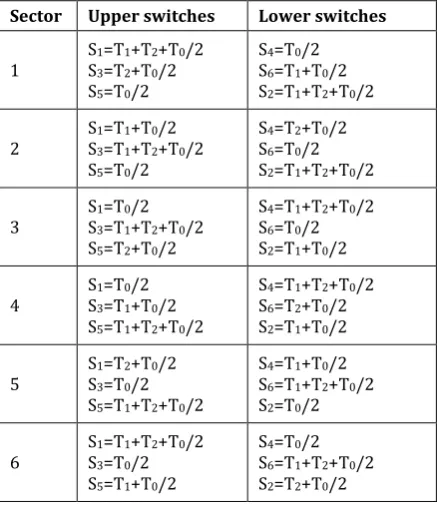
TABLE III. Switching time calculation at each sector.

Sector Upper switches Lower switches

1 SS13=T=T21+T+T20/2 +T0/2

S5=T0/2

S4=T0/2

S6=T1+T0/2

S2=T1+T2+T0/2

2 SS31=T=T11+T+T02/2 +T0/2

S5=T0/2

S4=T2+T0/2

S6=T0/2

S2=T1+T2+T0/2

3 SS13=T=T01/2 +T2+T0/2

S5=T2+T0/2

S4=T1+T2+T0/2

S6=T0/2

S2=T1+T0/2

4 SS13=T=T01/2 +T0/2

S5=T1+T2+T0/2

S4=T1+T2+T0/2

S6=T2+T0/2

S2=T1+T0/2

5 SS13=T=T20+T/2 0/2

S5=T1+T2+T0/2

S4=T1+T0/2

S6=T1+T2+T0/2

S2=T0/2

6 SS13=T=T10+T/2 2+T0/2

S5=T1+T0/2

S4=T0/2

S6=T1+T2+T0/2

S2=T2+T0/2

Duration of switching time at any sector is given by,

√ | |

( (

) ( ) ) (6)

√ | |

( (

( )

) (( ) ))

(7)

[image:2.595.45.285.423.625.2]

© 2017, IRJET | Impact Factor value: 6.171 | ISO 9001:2008 Certified Journal | Page 1115

III.

SLIDING MODE CONTROL (SMC)

Sliding-mode control (SMC) is the competent nonlinear control approaches which provide system dynamics that are controlled in the sliding mode. The first step is to choose a sliding surface which decides the desired closed-loop control performance as shown in [1]. Then design control is made to force the state trajectories close to the sliding surface and stay on it [5]. The trajectory of the system which slides along the sliding surface to its origin is said to be sliding mode [6]. Inertial weight, w is introduced in this control system to decide the applicable evolutionary length for accelerating the searching speed. Define a tracking error, e=d*-d, in which d* represents a specific position reference trajectory. The control nominal system dynamic is given by

̈ ̇ (9)

where k1 and k2 are positive constants. By properly choosing the values of k1 and k2, the desired system dynamic such as rise time, overshoot, and settling time can

be easily designed. The baseline model dynamic can be

rewritten in the state variable form as

* ̇+ = [ ]* ̇+ (10)

Or ̇ = where e =* _̇+ and A=[ ] (11)

Now consider the sliding surface as

S( ) ( ) ( ) ∫

Aed (12)

where ( ) is a scalar variable and is the initial state.

To sustain the state on the surface S(t)=0 for all time, one only needs to show that

( ) ̇( ) ,if ( ) (13)

When boundary layer is introduced around the sliding surface, the integral terms were used to eradicate steady-state error that results from continuous resemblance of switching control. Selection of proper boundary values makes the system dynamics to be stable. The significant effect on the control performance is the selection of upper bounds. Thus stability is achieved by using the sliding mode control (SMC) and it is then indirectly cinched into particle swarm optimization (PSO) to find optimized solution in the TSPSOC framework.

IV. PARTICLE SWARM OPTIMIZATION (PSO)

Particle swarm optimization is a progressive computation technique that was developed by Eberhart and Kennedy in 1995[7-17]. It is used for searching optimal by updating the generations. PSO is used as a minor compensatory tuner for controlling the speed but the stability of PSO control scheme cannot be guaranteed. The strategy for achieving the global version of PSO is given by the following steps [18][19][20].

 Initialize the population with random positions

and velocities in the n-dimensional problem space

using an uniform probability distribution function.

 Evaluate the fitness value of each particle.

According to the spirit of SMC, the ultimate evolutionary target of PSO can be regarded as S(t)=0 and S’(t)=0. Therefore, a fitness function is defined as

( ) [ ( ̇ )] [ ] (14)

Where exp[.] is the exponential function, η is a positive constant, and S is a sliding surface.

 Compare each particle’s fitness with the particle’s

lbest .If the fitness value of present particle position

is lower than the fitness values of local best particle position, the local best particle position should be modified by

( ) ( ) (15)

where n indicates the current state, n+1 means the next state, and δ is designed as a small positive constant to prevent the local optimum problem.

 Compare the fitness with the population’s overall

previous best.

 Change the velocity and position of the particle

according to [21] respectively.

( ) ( ) x w + c1 x rand(.) x [ ( ) ( )] x ̇

+c2 x rand(.) x[ ( ) ( )] x S (16)

where represents the particle velocity, rand(.)

is a random number between 0 and 1, c1 and c2 are the acceleration constants with positive values, w is an inertial weight and is defined as[8]

w=a+[ ( )] [ ( )] (17)

© 2017, IRJET | Impact Factor value: 6.171 | ISO 9001:2008 Certified Journal | Page 1116

position [22] will be calculated at the next time step according to the following equation:

( ) ( ) ( ) (18)

A.

Procedure Involved in PSO

In order to state the procedures involved in the design of a PSO-based control scheme, the flowchart of the proposed system is depicted. For easy to understand, it supposes that four particle positions (u1, u2, u3, u4) and the corresponding particle velocities (pv1, pv2, pv3, pv4) in the initial population (N=4) are randomly chosen from the

reasonable region [umin, umax].

Process 1: In steps 1 and step 2, the corresponding fitness values (FIT1, FIT2, FIT3, FIT4) are evaluated via immediate tracking responses in Step 3.

Process 2 : The first fitness value is regarded as the global best particle position by selecting the particle positions with the first and second fitness values from these four particles, and the second fitness value is applied as the local best particle position in Step 4.

Process 3 : u3 is chosen as the global best particle position (gbest (0)), and u4 is selected as the local best particle

position (lbest(0)).

Process 4 : The particle velocity and position is updated via Eqs. (3) and (5) in Step 10.

Process 5 : If the new particle position exceeds beyond the

boundary [umin, umax] as discussed in step 11, the new

particle position will be fixed as umin or umax (Step 12), else

it directly outputs the results of Eq. (5) as the new particle position. Then the new particle position is regarded as the new control effort to export as shown in Step 13.

Process 6 : After the first generation this new control effort will be treated as the current particle position of the next generation because it is the most suitable particle for the present circumstance.

Process 7 : If the fitness value of current particle position lies in between the fitness values of the global and local particle positions (Step 5), the current particle position will become the new local best particle position (Step 6).

Process 8 : If the fitness value of current particle position is higher than the global best fitness value, the current particle position will become the new global best particle position and the old global best particle position will replace the local best particle position (Step 8).

Process 9 : If the fitness value of current particle position is lower than the local best fitness value (Step 7), the local best particle position should be modified by Eq. (2) (Step 9).

B.

Flowchart

The operation process will repeat continuously until this program completes, so that adaptive control effort will be produced persistently .Consequently the objective of PSO control can be achieved and the stability of the proposed TSPSOC strategy can be indirectly clinched by means of the spirit of SMC. The process involved by PSO for finding the optimum solution is shown by using the flowchart

© 2017, IRJET | Impact Factor value: 6.171 | ISO 9001:2008 Certified Journal | Page 1117

V. V/F CONTROL

The constant V/F control method is the most popular method of scalar control. Here, supply frequency is set constant as 50 Hz and voltage is varied. Therefore the region below the base or rated frequency should be followed by the commensurate reduction of stator voltage so as to uphold the air gap flux constant. The torque and speed can be varied by varying the voltage and frequency. The torque is sustained constant while the speed is varied. The role of the volts hertz control is to uphold the air gap flux of AC induction motor constant in order to achieve higher run-time efficiency. The truancy of high in-rush starting current in a direct-start device reduces stress and therefore improves the effective life of machine.

VI. SIMULATION RESULTS

Simulation of induction motor with PSO and SMC is done by MATLAB/SIMULINK. The inverter voltage & frequency can be controlled by V/F method. The ratio of voltage and frequency have been maintained as constant. The speed and current are taken as feedback element and helps to maintain the ratio of V/F method. As shown in module Fig. 5, the speed has been set as set point while the actual speed is measured as feedback signal. The error and derivative of error are used as the input of SMC block. The tracking error is reduced by using the sliding mode controllers and the boundary layer was introduced around the sliding surface, in order to eliminate the steady-state error which results in a continuous approximation of switching control. This property is helpful for defining the corresponding fitness function and particle velocity to become a direction-based PSO algorithm.

[image:5.595.308.556.102.478.2]

The PSO control scheme is utilized to be the major controller, and the stability can be indirectly incorporatd by the concept of SMC without strict constraint and detailed system knowledge. The output of PSO is given to given to the space vector pulse width modulation. Parameters of induction motor which has tested with SMC and PSO is shown in table IV.

TABLE IV. Parameters of induction motor which has tested with PSO and SMC

Parameter Values

Power 5.4 hp (4 KW)

Rated Speed 1430 rpm

Type Squirrel cage

Voltage 400 V

Dc Link voltage (Vdc) 600 V

Stator Resistance (Rs) 1.405 Ω

Stator Inductance (Ls) 0.005839 H

Rotor Resistance (Rr) 1.395Ω

Rotor Inductance (Lr) 0.005839 H

Mutual Inductance(M) 0.1722 H

Number of Poles (P) 4

Inertia (J) 0.0131

Friction (B) 0.002985

[image:5.595.39.560.639.780.2]

Fig. 4. Simulink model of induction motor with PSO and SMC

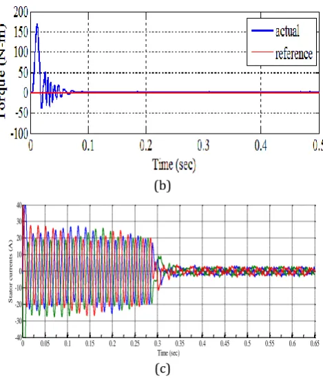
Initially the reference speed is set at 1000rpm. Fig 5 shows the starting characteristics of PSO and SMC with no load. When the motor runs at no-load the peak overshoot is lesser and the value is 0.37. The settling time is 0.4 sec.

At start, the time length of inrush current is up to 0.29 seconds. The Torque starts to reach the steady state at 0.06 second with lesser ripples and finally reaches the steady state at 0.09 sec without ripples.

(a)

0.32 0.34 0.36 0.38 0.4 0.42 0.44 0.46 0.48 0.5 0.52

900 950 1000 1050 1100

Time (sec)

S

p

e

e

d

(

rp

m

)

© 2017, IRJET | Impact Factor value: 6.171 | ISO 9001:2008 Certified Journal | Page 1118

(b)

[image:6.595.45.280.98.373.2]

(c)

Fig. 5. Dynamic response of IM with SMC and PSO at starting with no load. (a) Peak overshoots (b) Starting

[image:6.595.326.541.104.206.2]

Torque (c) Stator current

Fig. 6, shows the starting characteristics of SMC and PSO with slight load (1 N-m). The speed has been settled at 0.4 second. At start the time length of inrush current in SMC and PSO is up to 0.37 second. The Torque reaches the steady state at 0.38 second in SMC and PSO.

(a)

(b)

(c)

Fig. 6. Dynamic response IM with SMC and PSO at starting with load (1 N-m). (a)Peaks overshoot (b) stator current(c)

Starting Torque

(a)

(b)

(c)

Fig. 7. Dynamic response IM with SMC and PSO with sudden Load of 4N-m at t=1 sec. (a) Peak overshoot (b)

stator current (c) Starting Torque.

The load of 4 N-m is applied at t = 1 second suddenly. The Fig. 7 shows the transient response of SMC and PSO with sudden applied load at t=1 sec. The speed has been settled at 1.1 sec in PSO and SMC after the disturbances. The torque is uniform in SMC and PSO control.

The Fig. 8, shows the transient response of SMC and PSO with sudden increase in speed of 1200 rpm with the same load of 4 N-m at t=1.5sec. The speed is settled at 1.65 second in SMC and PSO control.

0 0.05 0.1 0.15 0.2 0.25 0.3 0.35 0.4 0.45 0.5 0.55 0.6 0.65

-40 -30 -20 -10 0 10 20 30 40 Time (sec) S ta to r c u r r e n ts ( A )

0.32 0.34 0.36 0.38 0.4 0.42 0.44 0.46 0.48 0.5 900 925 950 975 1000 1025 1050 1075 Time (sec) S p e e d ( r p m ) Actual speed Reference speed

0 0.05 0.1 0.15 0.2 0.25 0.3 0.35 0.4 0.45 0.5 0.55 0.6 -30 -20 -10 0 10 20 30 40 Time (sec) S ta to r c u r r e n ts ( A )

0 0.1 0.2 0.3 0.4 0.5 0.6 0.7 0.8 0.9 1

-45 -35 -25 -15 -5 5 15 25 35 45 Time (sec) T o rq u e ( N -m )

0.3 0.4 0.5 0.6 0.7 0.8 0.9 1 1.1 1.2 1.3 1.4 970 980 990 1000 1010 1020 Time (sec) S p e e d ( rp m ) Actual speed Reference speed

0 0.1 0.2 0.3 0.4 0.5 0.6 0.7 0.8 0.9 1 1.1 1.2 1.3 1.4 1.45

-50 -40 -30 -20 -10 0 10 20 30 40 50 Time (sec) S ta to r c u rr e n ts ( A )

0.4 0.5 0.6 0.7 0.8 0.9 1 1.1 1.2 1.3 1.4 1.5

[image:6.595.331.541.271.554.2] [image:6.595.66.281.494.730.2]

© 2017, IRJET | Impact Factor value: 6.171 | ISO 9001:2008 Certified Journal | Page 1119

(a)

(b)

(c)

Fig. 8. Transient response of IM with SMC and PSO, step change of speed 1200 rpm with load at t=1.5 sec. (a) Peak

overshoot (b) Torque (c) Stator current.

TABLE V. Performance in time domain analysis at no- load

Controller overshooPeak t (%)

Peak time (sec)

Rise time (sec)

Settle time (sec)

SMC and

[image:7.595.61.266.99.412.2]

PSO 0.35 0.353 0.344 0.4

TABLE VI. Performance in time domain analysis at load of 1 N-m

Controller Peak overshoo t (%)

Peak time (sec)

Rise time (sec)

Settle time (sec)

SMC and

PSO 0.38 0.358 0.348 0.4

TABLE V - TABLE VII shows the performance in time domain analysis with various load conditions. Fig. 5–Fig. 9 illustrate the performance of speed, torque, stator current and THD for induction motor using SVPWM technique in no load, slight load 1 N-m, load with 4 N-m at t=1sec and speed increases to 1200 rpm with load at 1.5 sec. The THD has been analyzed for stator current at t=1.2 second is shown

in Fig. 9.FLC controller shows 12.27% of THD in stator current.

TABLE VII. Performance in time domain analysis when the load increased to 1200 with the load of 4N-m

After the Sudden load

4 Nm applied at t=1s speed 1200 rpm at t=1.5s After the step change of with load

Settling time(sec) Settling time(sec)

PSO and SMC controller PSO and SMC controller

1.1 1.62

Fig. 9. T.H.D of stator current at t = 1.2 sec with frequency 37.5 Hz of SMC and PSO controller.

VII. CONCLUSION

This proposal of speed control of an AC drive using sliding mode control and particle swarm optimization controller with SVPWM shows swift, downy, and high dynamic response. 80 % of speed is achieved by tuning PSO parameters using space vector pulse width modulation. The stability of system dynamics is achieved by sliding mode control which reduces the steady state error by continuous switching. The MATLAB software is tested for the entire closed loop control of Induction motor using PWM techniques with particle swarm optimization (PSO) and sliding mode control. The performance of a system with variable load and the speed is good. The controller gives uniform torque and the THD value for stator current is 12.27%. The FFT analysis window shows that the

magnitude of fractional harmonics between 0 and 1, 1st _and

2nd _{order is lower in SMC and PSO. Thus I came to the}

conclusion that the PSO and SMC controller with SVPWM gives improved performance for AC drives.

1.2 1.3 1.4 1.5 1.6 1.7 1.8 1.9 2

950 1000 1050 1100 1150 1200 1250 1300

Time (sec)

S

p

e

e

d

(

rp

m

)

1 1.1 1.2 1.3 1.4 1.5 1.6 1.7 1.8 1.9 2

-10 -5 0 5 10 15 20

Time (sec)

T

o

rq

u

e

(

N

-m

)

0 0.2 0.4 0.6 0.8 1 1.2 1.4

0 50 100

Selected signal: 52.5 cycles. FFT window (in red): 3 cycles

Time (s)

0 0.5 1 1.5 2 2.5 3 3.5 4 4.5 5 0

20 40 60 80 100

Harmonic order Fundamental (37.5Hz) = 6.096 , THD= 12.27%

M

a

g

(

%

o

f

F

u

n

d

a

m

e

n

t

a

l

[image:7.595.308.557.166.448.2]

© 2017, IRJET | Impact Factor value: 6.171 | ISO 9001:2008 Certified Journal | Page 1120

REFERENCES

[1]Rong-Jong Wain, Yeou-Fu Lin, Kun-Lun Chuang, “Total

sliding-mode-based particle swarm optimization

control for linear induction motor”,

www.elsevier.com/locate/jfranklin, Journal of the

franklin institute 351 (2014) 2755–2780.

[2]Divya Rai, Swati Sharma, Vijay Bhuria, “Fuzzy speed

controller design of three phase induction

motor”,International Journal of Emerging Technology and Advanced Engineering, ISSN 2250-2459, Volume 2, Issue 5, May 2012.

[3] V.Vengatesan, M.Chindamani, “Speed Control of Three

Phase Induction Motor using Fuzzy Logic Controller by Space Vector Modulation Technique”, International Journal of Advanced Research in Electrical, Electronics and Instrumentation Engineering, ISSN 2320-3765 Vol. 3, Issue 12, December 2014.

[4]B. K. Bose, Modern Power Electronics and AC Drive,

Prentice Hall, 2002, PP.63-70.

[5]RIOS-BOLIVAR, M., and ZINOBER, A.S.I.: 'Dynamical

adaptive sliding mode control of observable minimum-phase urlcerlain non- linear systems'. in 'Variable Structure Systems, Sliding Mode and Nonlinear Control' (Springer-Veilag. Londan. UK, 1999),pp. 211-235.

[6]RARTOLINI. G.. FERRARA. A,, GIACOMINI. L.. and USAI,

E.: 'Properties of a combined adeptivc/smond-order sliding modc control algorithm for some classes of uncertain nonlinear systems', IEEE Trun.. Auro. Conrrol, 2000, 45, (7). pp. 1334-1341

[7]R.C. Eberhart, J. Kennedy, A new optimizer using

particles swarm theory, in: Proceedings of the Sixth International Symposium on Micro Machine and Human Science, 1995, pp. 39–43.

[8] R.C. Eberhart, J. Kennedy, Particle swarm optimization, in: Proceedings of the IEEE Conference on Neural Networks, 1995, pp. 1942–1948.

[9] Y. Shi, R.C. Eberhart, A modified particle swarm optimizer, in: Proceedings of the IEEE Conference on Computation Intelligence, 1998, pp. 69–73.

[10] S.H. Ling, H.H.C. Iu, F.H.F. Leung, K.Y. Chan, Improved hybrid particle swarm optimized wavelet neural network for modeling the development of fluid dispensing for electronic packaging, IEEE Trans. Ind. Electron. 55 (9) (2008) 3447–3460.

[11] L.S. Coelho, B.M. Herrera, Fuzzy identification based on a chaotic particle swarm optimization approach applied toa nonlinear yo-yo motion system, IEEE Trans. Ind. Electron. 54 (6) (2007) 3234–3245.

[12] H.M. Feng, Self-generation RBFNs using evolutional PSO learning, Neurocomputing 70 (2006) 241–251.

[13] A.Chatterjee, K. Pulasinghe, K. Watanabe, K. Izumi, A particle-swarm-optimized fuzzy-neural network for voice controlled robot systems, IEEE Trans. Ind. Electron. 52 (6) (2005) 1478–1489.

[14] S. Panda, B.K. Sahu, P.K. Mohanty, Design and performance analysis of PID controller for an automatic voltage regulator system using simplified particle swarm optimization, J. Frankl. Inst. 349 (2012) 2609– 2625.

[15] F.J. Lin, L.T. Teng, H. Chu, Modified Elman neural network controller with improved particle swarm optimisation for linear synchronous motor drive, IET Electr. Power Appl. 2 (3) (2008) 201–214.

[16] R.-J. Wai et al. / Journal of the Franklin Institute 351 (2014) 2755–2780 2779

[17] K.W. Yu, S.C. Hu, An application of AC servo motor by using particle swarm optimization based sliding mode controller, in: Proceedings of the IEEE Conference on Systems, Man, and Cybernetics, 2006, pp. 4146–4150.

[18] R. A. Krohling and L. S. Coelho, “Coevolutionary particle swarm optimization using Gaussian distribution for solving constrained optimization problems,” IEEE Trans. Syst., Man Cybern. B, Cybern., vol. 36, no. 6,pp. 1407–1416, Dec. 2006.

[19] A.Karimi, A. Feliachi, Decentralized adaptive backstepping control of electric power system, Electr. Power Syst.Res. 78 (3) (2008) 484–493.

[20] R. A. Krohling, F. Hoffmann, and L. S. Coelho, “Co-evolutionary particle swarm optimization for min–max problems using Gaussian distribution,”in Proc. Congr. Evol. Comput., Portland, OR, 2004, pp. 959–964.

[21] Y. Shi and R. C. Eberhart, “A modified particle swarm optimiser,” in Proc.IEEE World Congr. Comput. Intel., Evol. Comput., Anchorage, AL, 1998,pp. 69–73.