http://dx.doi.org/10.4236/ojab.2014.34004
An Efficient and Robust Fall Detection
System Using Wireless Gait Analysis Sensor
with Artificial Neural Network (ANN) and
Support Vector Machine (SVM) Algorithms
Bhargava Teja Nukala
1, Naohiro Shibuya
1,2, Amanda Rodriguez
3, Jerry Tsay
1,
Jerry Lopez
1, Tam Nguyen
1,3, Steven Zupancic
3, Donald Yu-Chun Lie
1,3 1Texas Tech University (TTU), Lubbock, USA2(On Leave) The Department Electrical & Electronic Engineering, Tokushima University, Tokushima, Japan 3Texas Tech University Health Sciences Center (TTUHSC), Lubbock, USA
Email: [email protected]
Received 28 September 2014; revised 26 October 2014; accepted 5 November 2014
Copyright © 2014 by authors and Scientific Research Publishing Inc.
This work is licensed under the Creative Commons Attribution International License (CC BY).
http://creativecommons.org/licenses/by/4.0/
Abstract
In this work, a total of 322 tests were taken on young volunteers by performing 10 different falls, 6 different Activities of Daily Living (ADL) and 7 Dynamic Gait Index (DGI) tests using a custom-de- signed Wireless Gait Analysis Sensor (WGAS). In order to perform automatic fall detection, we used Back Propagation Artificial Neural Network (BP-ANN) and Support Vector Machine (SVM) based on the 6 features extracted from the raw data. The WGAS, which includes a tri-axial accele-rometer, 2 gyroscopes, and a MSP430 microcontroller, is worn by the subjects at either T4 (at back) or as a belt-clip in front of the waist during the various tests. The raw data is wirelessly transmit-ted from the WGAS to a near-by PC for real-time fall classification. The BP ANN is optimized by vary- ing the training, testing and validation data sets and training the network with different learning schemes. SVM is optimized by using three different kernels and selecting the kernel for best classi- fication rate. The overall accuracy of BP ANN is obtained as 98.20% with LM and RPROP training from the T4 data, while from the data taken at the belt, we achieved 98.70% with LM and SCG learning. The overall accuracy using SVM was 98.80% and 98.71% with RBF kernel from the T4 and belt position data, respectively.
Keywords
1. Introduction
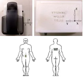
It is estimated that one third of the senior citizens in the United States (i.e., around 12 million people) fall each year, which often results in serious injuries [1]. Falls in elderly persons living alone can be especially dangerous. Therefore, it is important to introduce a highly accurate and easy-to-wear fall detection device that can wire-lessly detect and record real-time falls for the aging population. We have performed investigation using our custom sensor without the wireless feature and achieved 100% accuracy in identifying all 60 falls vs. the Activi-ties of Daily Living (ADL) with no false positives on young volunteers using threshold based algorithms [2]. For this current work, the sensor is wireless and allows for real-time untethered testing for not only fall detec-tions, but also for gait analysis [2] [3]. This paper reports our new Wireless Gait Analysis Sensor (WGAS) used specifically for real-time automatic fall detection with an efficient Back Propagation Artificial Neural Network (BP ANN) algorithm with different training schemes and Support Vector Machine (SVM) with different kernel functions. This WGAS is placed and tested at two different positions on the body: at the T4 position and at the Belt position using a belt clip as shown in Figure 1.
For the learning of BP ANN and SVM, the following 6 features (Rω: Range of angular velocity; RA: Range
of acceleration) as shown in Equations (1) and (2) were extracted from the raw data taken from WGAS. They are used to perform real-time fall detection as supplied as inputs to these classifiers.
( )
( )
( )
( )
( )
( )
,x max x min x , ,y max y min y , ,z max z min z ,
Rω = ω − ω Rω = ω − ω Rω = ω − ω (1)
( )
( )
( )
( )
( )
( )
, max min , , max min , , max min .
A x x x A y y y A z z z
R = A − A R = A − A R = A − A (2)
2. Wireless Gait Analysis Sensor
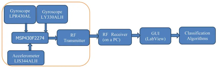
The custom-designed WGAS consists of a 3-axis linear accelerometer, a single axis gyroscope, and a dual axis gyroscope to measure 3-D human body translations and rotations during a gait pattern with the help of the Micro- Electrical and Mechanical System (MEMS) sensors integrated on a PCB. This WGAS system is supported by a Texas Instruments (TI) MSP430 microcontroller, and a wireless 2.4 GHz USB transceiver using the SimpliciTI™ protocol with a range of ~12 meters (40 ft). An overall simplified system block diagram for the WGAS fall detec-tion system is shown in Figure 2. The 2 AAA batteries used in our earlier wired sensor [2] were replaced by
[image:2.595.164.436.442.695.2]
Figure 1. Sensor orientation and location at the belt position on a belt clip
Figure 2. A simplified block diagram of the WGAS fall detection system.
a single rechargeable Li-ion coin battery, providing a battery lifetime of ~40 hours continuous operation time with each recharge. The PCB, coin battery and the microcontroller are placed in a specially designed 3D printed box
(
2.2′×1.5′×0.8′)
with a total weight of 42 grams. The design of the box was done with a 3D modeling software Rhinoceros (Rhino) and printed using a 3D printer with Acrylonitrile Butadiene Styrene (ABS) plastic. The box has a sliding lid and shown in Figure 3.The accelerometer data is sampled at 160 Hz and digitized to 8 bits, with its output scaled to ±6 g at ΔV = ±6 g VDD
(
VDD =3.6 V)
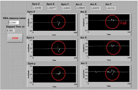
for each axis. The gyroscope data is also sampled at 160 Hz and digitized to 8bits, with its output scaled to 300˚ per sec. (dps) at ΔV = ±300 dps So (Note the typical So (sensitivity) value is 3.752 mV/dps for the accelerometer and 3.33 mV/dps for the gyroscopes). The sensor orientation and positions on the body are shown in Figure 1. The sensor is carefully secured to the subjects during testing to avoid artifacts. The microcontroller and the transceiver unit enables the real-time transmission of the 6-dimen- sional gait data wirelessly to the nearby PC, where a LABVIEW™ program is used for designing the Graphical User Interface (GUI) (Figure 4).
Testing Protocol
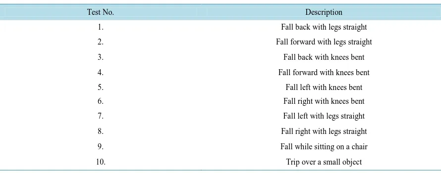
First falls [4] were performed on a cushion mattress bed by two young volunteers wearing the WGAS at T4 and on the belt (see Table 1 with 10 types of falls). The total number of falls was 101 (51 at T4 and 50 at belt). For the ADL tests [4], same volunteers performed every ADL recorded in Table 2 (note this includes picking up an object test #7), and the aggregate number of ADLs was 69 (34 at T4 and 35 at belt). For the DGI tests [5], the same volunteers performed every DGI test in Table 3, with 152 tests taken in total (82 at T4 and 70 at belt).
3. BP ANN Algorithm
For training the feed-forward ANN classifier, back propagation was applied according to Duda et al. [6] and a 3- layer system was picked as the standard BP ANN [7]. The input layer of the network has six neurons which cor-respond to the six input feature values. There is one hidden layer holding 10 hidden neurons, which number was optimized by adjusting the size of hidden neurons (from one to 15) as shown in Figure 5, where two output neurons corresponding to the two target classes the network needs to differentiate (i.e., the features of all falls are considered as Class 1, and all DGI and ADL are as Class 2). The essential idea of the back propagation learning algorithm [8] is the repeated application of the chain rule to calculate the impact of each weight in the network by taking an arbitrary error function E in to account as shown in Equation (3):
i i
ij i i ij
s net
E E
w s net w
∂ ∂
∂ ∂
=
∂ ∂ ∂ ∂ (3)
where wij is the weight from neuron j to neuron i, si is the output, and neti is the weighted sum of the inputs of
the neuron i. After calculating the derivative of each weight, the error function is minimized by following a simple gradient decent rule in Equation (4):
(
1)
( )
( )
ij ij
ij
E
w t w t t
w
ε ∂
+ = −
Figure 3. Physical structure of our custom-designed WGAS.
Figure 4. GUI designed in LABVIEWTM for our real-time fall detection system using the WGAS, indicating a fall occurred
[image:4.595.88.541.401.696.2]W
b
+
+
W
b
+
+
Input
Hidden Layer Output Layer
Output
10 2
[image:5.595.159.445.86.192.2]2 6
[image:5.595.87.532.233.408.2]Figure 5. The 3-layer BP ANN topology used in this work.
Table 1. Intentional falls performed in this work.
Test No. Description 1. Fall back with legs straight 2. Fall forward with legs straight 3. Fall back with knees bent 4. Fall forward with knees bent 5. Fall left with knees bent 6. Fall right with knees bent 7. Fall left with legs straight 8. Fall right with legs straight 9. Fall while sitting on a chair 10. Trip over a small object
Table 2. Activities of Daily Living (ADL) movements performed.
Test No. Description
1. Sitting down and standing up from an armchair 2. Sitting down and standing up from a low stool 3. Sitting down and standing up from a bed 4. Lying down and standing up from a bed 5. Walking 10 m
6. Stretching while standing 7. Picking up an object from the floor
Table 3. Dynamic Gait Index (DGI) tests performed.
Test No. Description 1. Gait level surface-walk with the normal speed up to 20' mark
2. Change in Gait speed-walk with normal pace up to 5', walk fast for next 5', walk slowly for next 5' and walk normal for last 5'
3. Gait with horizontal head turns-walk normal with horizontal head turns up to 20' mark 4. Gait with vertical head turns-walk normal with vertical head turns up to 20' mark 5. Gait and pivot turn-walk normal but at the end turn around like a pivot turn
6. Step over obstacle-walk normal and when you come across obstacle step over not around 7. Step around obstacles-walk normal and when 1st obstacle comes across, walk around right
Clearly, the decision of the learning rate ε, which scales the derivative, has a critical impact on the time re-quired until convergence is arrived. If the learning rate is set too small, numerous steps are expected to achieve an acceptable solution. On the contrary, a large learning rate will possibly lead to oscillation, preventing the error to fall below a certain value. The training of the BP ANN is done by using three different learning algorithms dis- cussed below.
3.1. BP ANN with Scaled Conjugate Gradient (SCG) Learning
The basic back propagation algorithm alters the weights of the network following the steepest descent direc-tion (negative direcdirec-tion of the slope). In this direcdirec-tion the performance funcdirec-tion decreases most rapidly along the negative direction of slope. However, convergence may not be achieved even though the decrease is more rapid. Therefore, conjugate gradient methods are used which can generally produce faster convergence than gradient descent techniques by performing a search in all the gradient directions to determine the step size obtained by the learning factor. The training of the ANN classifier used in this work is done by the scaled conjugate gradient (SCG) back propagation method developed by Moller [9]. This SCG algorithm performs the search and chooses the step size by using the information from the second order error function from the neural network. The SCG training is optimized by the parameter sigma σ (which determines the change in weight for the second derivative approximation) and lamda λ (which regulates the indefiniteness of the Hessian). The values of σ and λ were taken as 5 e⋅ −5 and 5 e⋅ −7, respectively.
3.2. BP ANN with Levenberg-Marquardt (LM) Learning
The second training method for BP ANN is done by the Levenberg-Marquardt algorithm [10], which is used to speed up the training of second order approximations without having to calculate the Hessian matrix. If the per-formance function has the sum of squares (typical in training feed-forward networks) then the Hessian matrix can be approximated as:
T
H=J ⋅J (5)
And the gradient can be calculated as
T
g=J ⋅e (6) where J is the Jacobian matrix, which has the first derivatives of the network errors with respect to the weights and biases, and e is a vector that contains the network errors.
To make sure the H is always invertible, the LM algorithm introduces another approximation to the Hessian matrix using.
T
H=J ⋅ + ⋅J µ I (7) where µ is called combination coefficient and is always positive and I is the identity matrix. The LM algorithm does the training according the scalar parameter µ. If the value of µ is zero, this algorithm reduces to the Hessian matrix approximation; and if the value of µ is large, this becomes a gradient descent algorithm with small step size. The LM training is optimized by the parameter µ (i.e., the combination coefficient). As µ can either be small or large, its value is initialized to 0.001 and the maximum value is set to 1 e⋅ 10, with a decrease factor of 0.1 and an increase factor of 10.
3.3. BP ANN with Resilient Propagation (RPROP)
4. Support Vector Machine (SVM)
Support Vector Machine (SVM) is a method for patterns recognition/classification on two categories with su-pervised learning. SVM-light, one of the implementation of SVM proposed by Thorsten Joachims [12] [13], is applied to classification of experimental data into falls, DGI and ADL.
4.1. Linear SVM Classification
The optimization algorithm for linear classification was proposed by Vapnik [14]. This algorithm finds the maxi- mum-margin hyper-plane from given training data set D as described in Equation (8):
(
)
{
}
{
, , 1,1}
1n p
i i i i
i
D y y
=
= x x ∈ ∈ − (8)
where yi is either 1 or 1 and n is the number of training data. Each xi is a p-dimensional vector having the fea- ture quantity . Any hyper-plane can be written as:
0 b
⋅ − =
w x (9)
where w is the vector to the hyper-plane. If the training data are linearly separable, the hyper-plane can be de-scribed as:
1 and 1.
b b
⋅ − = ⋅ − = −
w x w x (10)
The distance between these two hyper-plane is 2 w , so the purpose is to minimize w . Therefore, the al-gorithm can be rewritten as:
(
)
Minimize : w , under the condition of yi w x⋅ −i b ≥1, for any 1≤ ≤i n (11) We can also reformulate the equation without changing the solution as following:
( )
(
)
2
, , under the condition o 1
arg min
2 f i 1, for any 1
b y ⋅ −i b ≥ ≤ ≤i n
w w w x (12)
In Linear SVM, a hyper-plane or a set of hyper-planes can be used as the separate lines in classification. The higher the margin of separation for the classes that can be created, the better the classification result that can generally be achieved for the Linear SVM [15].
4.2. Nonlinear SVM Classification
B. E. Boser et al. proposed the nonlinear SVM classifiers by using the kernel trick [16]. The kernel functions used in this study are as followed:
(
) (
)
Polynomial :k x xi, j = x xi, j+1 .d (13)
(
)
(
2)
Radial Basis Function :k x xi, j =exp −γ x xi, j ,γ >0 (14)
The accuracy of SVM depends on the kernel, cost factor parameter C [17] and the parameter γ for the RBF kernel. We checked each combination of parameter choices in this work, and looked up for the best accuracy.
4.3. Overall Data Analysis Flow-Chart
After getting the raw data from the WGAS, feature extraction is performed by extracting 6 features as shown in Equations (1)-(2) and the training algorithms are implemented to obtain the fall detection.Figure 6 shows the complete data analysis flow chart of the WGAS system.
5. Classification Results
5.1. Classification Results Using the BP ANN Algorithm
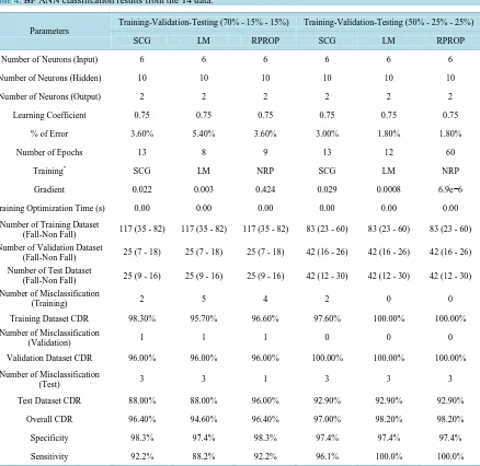
R2013b for the BP ANN classifier model. For the trained BP ANN classifier model, the number of training, va-lidation and testing data sets were divided into 70-15-15 and 50-25-25 in percentages, respectively for all the three training schemes. The classification results of SCG, LM and RPROP training schemes are shown in the Table 4 and Table 5. From Table 4 for the data at T4, LM and RPROP obtained the best overall Correct Detec-tion Rate (CDR) of 98.2% for the training-validaDetec-tion-testing (50% - 25% - 25%) data sets. And at the belt posi-tion from Table 5, LM yielded an overall CDR of 98.70% for the training-validation-testing (70% - 15% - 15%) data sets, and SCG yielded an overall CDR of 98.70% for the training-validation-testing (50% - 25% - 25%) data sets.
Figure 6. The data analysis flow-chart of the WGAS fall detection system.
Table 4. BP ANN classification results from the T4 data.
Parameters
Training-Validation-Testing (70% - 15% - 15%) Training-Validation-Testing (50% - 25% - 25%) SCG LM RPROP SCG LM RPROP Number of Neurons (Input) 6 6 6 6 6 6 Number of Neurons (Hidden) 10 10 10 10 10 10
Number of Neurons (Output) 2 2 2 2 2 2 Learning Coefficient 0.75 0.75 0.75 0.75 0.75 0.75
% of Error 3.60% 5.40% 3.60% 3.00% 1.80% 1.80% Number of Epochs 13 8 9 13 12 60
Training* SCG LM NRP SCG LM NRP
Gradient 0.022 0.003 0.424 0.029 0.0008 6.9e−6 Training Optimization Time (s) 0.00 0.00 0.00 0.00 0.00 0.00
Number of Training Dataset
(Fall-Non Fall) 117 (35 - 82) 117 (35 - 82) 117 (35 - 82) 83 (23 - 60) 83 (23 - 60) 83 (23 - 60) Number of Validation Dataset
(Fall-Non Fall) 25 (7 - 18) 25 (7 - 18) 25 (7 - 18) 42 (16 - 26) 42 (16 - 26) 42 (16 - 26) Number of Test Dataset
(Fall-Non Fall) 25 (9 - 16) 25 (9 - 16) 25 (9 - 16) 42 (12 - 30) 42 (12 - 30) 42 (12 - 30) Number of Misclassification
(Training) 2 5 4 2 0 0 Training Dataset CDR 98.30% 95.70% 96.60% 97.60% 100.00% 100.00% Number of Misclassification
(Validation) 1 1 1 0 0 0 Validation Dataset CDR 96.00% 96.00% 96.00% 100.00% 100.00% 100.00% Number of Misclassification
(Test) 3 3 1 3 3 3 Test Dataset CDR 88.00% 88.00% 96.00% 92.90% 92.90% 92.90%
Overall CDR 96.40% 94.60% 96.40% 97.00% 98.20% 98.20% Specificity 98.3% 97.4% 98.3% 97.4% 97.4% 97.4% Sensitivity 92.2% 88.2% 92.2% 96.1% 100.0% 100.0%
*
Table 5. BP ANN classification results from the belt position data.
Parameters Training-Validation-Testing (70% - 15% - 15%) Training-Validation-Testing (50% - 25% - 25%) SCG LM RPROP SCG LM RPROP Number of Neurons (Input) 6 6 6 6 6 6 Number of Neurons (Hidden) 10 10 10 10 10 10 Number of Neurons (Output) 2 2 2 2 2 2
Learning Coefficient 0.75 0.75 0.75 0.75 0.75 0.75 % of Error 1.90% 1.30% 3.20% 1.30% 8.40% 2.60% Number of Epochs 14 11 12 17 8 14
Training* SCG LM RP SCG LM NRP
Gradient 0.0064 0.0022 0.043 0.007 0.0037 0.0416 Training Optimization Time (s) 0.00 0.00 0.00 0.00 0.00 0.00
Number of Training Dataset
(Fall-Non Fall) 109 (36 - 73) 109 (36 - 73) 109 (36 - 73) 77 (28 - 49) 77 (28 - 49) 77 (28 - 49) Number of Validation Dataset
(Fall-Non Fall) 23 (7 - 16) 23 (7 - 16) 23 (7 - 16) 39 (12 - 27) 39 (12 - 27) 39 (12 - 27) Number of Test Dataset
(Fall-Non Fall) 23 (7 - 16) 23 (7 - 16) 23 (7 - 16) 39 (10 - 29) 39 (10 - 29) 39 (10 - 29) Number of Misclassification
(Training) 0 0 2 0 7 0 Training Dataset CDR 100.00% 100.00% 98.20% 100.00% 90.90% 100.00% Number of Misclassification
(Validation) 3 2 2 2 2 2 Validation Dataset CDR 87.00% 91.30% 91.30% 94.90% 94.90% 94.90% Number of Misclassification
(Test) 0 0 1 0 4 2 Test Dataset CDR 100.00% 100.00% 95.70% 100.00% 89.70% 94.90%
Overall CDR 98.10% 98.70% 96.80% 98.70% 91.60% 97.40% Specificity 100.0% 100.0% 98.1% 100.0% 87.6% 98.1% Sensitivity 94.0% 96.0% 94.0% 96.0% 100.0% 96.0%
*
SCG: scaled conjugate gradient; LM: levenberg-marquardt; RP: resilient propagation.
The performance indicators such as specificity and sensitivity were also calculated by using Equations (14)- (15) and shown in Table 4 and Table 5.
TN Specificity
TN FP
=
+ (15)
TP Sensitivity
TP FN
=
+ (16)
where TN (true negatives) are the ADLs and DGIs correctly classified, FP (false positives) are the ADLs and DGIs that were not correctly classified by the BP ANN/SVM; TP (true positives) are the falls correctly classi-fied and FN (false negatives) are the falls that were not detected by the BP ANN/SVM.
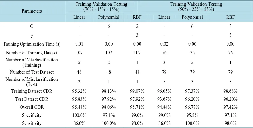
5.2. Classification Results Using the SVM Algorithm
Table 6. SVM classification results from the T4 data.
Parameters
Training-Validation-Testing (70% - 15% - 15%)
Training-Validation-Testing (50% - 25% - 25%) Linear Polynomial RBF Linear Polynomial RBF C - 2 1 - 2 1
γ - - 3 - - 3 Training Optimization Time (s) 0.01 0.00 0.00 0.01 0.00 0.00
Number of Training Dataset 115 115 115 81 81 81 Number of Misclassification (Training) 4 1 1 5 1 1
Number of Test Dataset 52 52 52 86 86 86 Number of Misclassification (Test) 5 4 3 5 5 2
Training Dataset CDR 96.52% 99.13% 99.13% 93.83% 98.77% 98.77% Test Dataset CDR 90.38% 92.31% 98.08% 94.19% 94.19% 97.67% Overall CDR 94.61% 97.01% 98.80% 94.01% 96.40% 98.20% Specificity 98.3% 99.1% 99.1% 98.3% 98.3% 100.0% Sensitivity 86.3% 92.2% 94.1% 84.3% 92.2% 94.1%
*
[image:10.595.90.534.348.573.2]RBF: radial basis function.
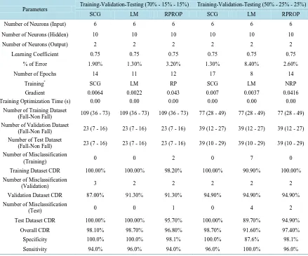
Table 7. SVM classification results from the belt position data.
Parameters
Training-Validation-Testing (70% - 15% - 15%)
Training-Validation-Testing (50% - 25% - 25%)
Linear Polynomial RBF Linear Polynomial RBF
C - 6 2 - 6 3
γ - - 3 - - 3 Training Optimization Time (s) 0.01 0.00 0.00 0.02 0.00 0.00
Number of Training Dataset 107 107 107 76 76 76 Number of Misclassification
(Training) 5 2 1 3 2 1 Number of Test Dataset 48 48 48 79 79 79 Number of Misclassification
(Test) 2 1 1 5 3 3 Training Dataset CDR 95.32% 98.13% 99.07% 96.05% 97.37% 98.68%
Test Dataset CDR 95.83% 97.92% 97.92% 93.67% 96.20% 96.20% Overall CDR 95.48% 98.06% 98.71% 94.84% 96.77% 97.42% Specificity 100.0% 97.1% 99.0% 99.0% 95.2% 97.1% Sensitivity 86.0% 100.0% 98.0% 86.0% 100.0% 98.0%
*RBF: radial basis function.
Table 6. From Table 7, we achieved 98.71% CDR at the belt position for training-validation-testing (70% - 15% - 15%) data sets by the RBF kernel.
6. Conclusions
highest sensitivity of 94.1% at the T4 position. The Linear kernel SVM has the highest specificity of 100%, and the Polynomial kernel SVM has the highest sensitivity of 100%. Overall, the SVM shows a slightly lower sensi-tivity than the BP ANN. This is likely because the SVM uses an RBF kernel as the activation function, whereas the BP ANN uses a tan sigmoid (Tanh) function that has better recognition accuracy.
The preliminary data that was collected on the group of young volunteers reported here suggests that our real- time fall detection system performs competitively regardless if the WGAS is placed at the T4 or waist-level Belt position. The application of the WGAS is not only useful for the fall detection, but also for the gait analysis. However, to make our fall detection work to be clinically relevant, a bit more data should be collected during clinical trials at TTUHSC in order to carefully evaluate the performance of the classifiers and their classification accuracies using the WGAS on patients. Our WGAS has passed the TTUHSC IRB (Internal Review Board), and is going through clinical trials on patients with balance disorders. The initial results look rather promising for gaits differentiation.
References
[1] Centers for Disease Control and Prevention (2015) Falls among Older Adults: An Overview.
http://www.cdc.gov/homeandrecreationalsafety/falls/adultfalls.html
[2] Jacob, J., Nguyen, T., Zupancic, S. and Lie, D.Y.C. (2011) A Fall Detection Study on the Sensor Placement Locations and the Development of a Threshold-Based Algorithm Using Both Accelerometer and Gyroscope. Proceedings of IEEE International Conference on Fuzzy Logics, Taipei, 27-30 June 2011, 666-671.
[3] Nukala, B.T., Rodriguez, A.I., Tsay, J., Hall, T., Nguyen, T.Q., Zupancic, S. and Lie, D.Y.C. (2014) Evaluating Op-timal Placement of Real-Time Wireless Gait Analysis Sensor with Dynamic Gait Index (DGI). Actas IEEE Conference on Information Systems and Techno (CISTI), Barcelona, 18-21 June 2014, 160-161.
[4] Narasimhan, R. (2012) Skin-Contact Sensor for Automatic Fall Detection. Proceedings of IEEE International En-gineering in Medicine and Biology Society (EMBS) Conference, San Diego, 28 August-1 September 2012, 4038-4041.
[5] Perel, K.L., Nelson, A., Goldman, R.L., Luther, S.L., Prieto-Lewis, N. and Rubenstein, L.Z. (2001) Fall Risk Assess-ment Measures: An Analytic Review. Journals of Gerontology Series A—Biological Sciences & Medical Sciences, 56, M761-M766. http://dx.doi.org/10.1093/gerona/56.12.M761
[6] Duda, R.O., Hart, P.E. and Stork, D.G. (2001) Pattern Classification. 2nd Edition, Wiley-Interscience, New York. [7] Dreiseitl, S. and Ohno-Machado, L. (2002) Logistic Regression and Artificial Neural Network Classification Models:
A Methodology Review. Journal of Biomedical Informatics, 35, 352-359.
http://dx.doi.org/10.1016/S1532-0464(03)00034-0
[8] Rumelhart, D.E., Hinton, G.E. and Williams, R.J. (1985) Learning Internal Representations by Error Propagation. In: Rumelhart, D.E. and McClelland, J.L., The PDP Group, Eds., Parallel Distributed Processing: Explorations in the Mi-crostructure of Cognition, Volume 1, Foundations, MIT Press, Cambridge, 318-362.
[9] Moller, M.F. (1993) A Scaled Conjugate Gradient Algorithm for Fast Supervised Learning. Neural Networks, 6, 525- 533. http://dx.doi.org/10.1016/S0893-6080(05)80056-5
[10] Marquardt, D. (1963) An Algorithm for Least-Squares Estimation of Nonlinear Parameters. SIAM Journal on Applied Mathematics, 11, 431-441. http://dx.doi.org/10.1137/0111030
[11] Riedmiller, M. and Braun, H. (1993) A Direct Adaptive Method for Faster Backpropagation Learning: The RPROP Algorithm. IEEE International Conference on Neural Networks, 1, 586-591.
http://dx.doi.org/10.1109/ICNN.1993.298623
[12] Joachims, T. (2008) SVMLight Support Vector Machine. http://svmlight.joachims.org/
[13] Joachims, T. (1999) Making Large-Scale Support Vector Machine Learning Practical. In: Schölkopf, B., Burges, C.J.C. and Smola, A.J., Eds., Advances in Kernel Methods—Support Vector Learning, MIT Press, Cambridge, 169-184.
[14] Cortes, C. and Vapnik, V. (1995) Support-Vector Networks. Machine Learning, 20, 273-297.
http://dx.doi.org/10.1007/BF00994018
[15] Burges, C.J.C. (1998) A Tutorial on Support Vector Machines for Pattern Recognition. Data Mining and Knowledge Discovery, 2, 121-167.
[16] Boser, B.E., Guyon, I.M. and Vapnik, V.N. (1992) A Training Algorithm for Optimal Margin Classifiers. Proceedings of the 5th Annual Workshop on Computational Learning Theory (COLT’92), Pittsburgh, 27-29 July 1992, 144-152.