www.hydrol-earth-syst-sci.net/19/657/2015/ doi:10.5194/hess-19-657-2015
© Author(s) 2015. CC Attribution 3.0 License.
Drivers of spatial and temporal variability of streamflow in the
Incomati River basin
A. M. L. Saraiva Okello1,3, I. Masih1, S. Uhlenbrook1,2, G. P. W. Jewitt3, P. van der Zaag1,2, and E. Riddell3
1UNESCO-IHE, Institute for Water Education, P.O. Box 3015, 2601 DA Delft, the Netherlands
2Delft University of Technology, Department of Water Resources, P.O. Box 5048, 2600 GA Delft, the Netherlands 3Centre for Water Resources Research, School of Agriculture, Earth and Environmental Science,
University of KwaZulu-Natal, Private Bag X01, Scottsville, 3209, South Africa Correspondence to: A. M. L. Saraiva Okello ([email protected])
Received: 16 June 2014 – Published in Hydrol. Earth Syst. Sci. Discuss.: 29 July 2014 Revised: – – Accepted: 5 January 2015 – Published: 2 February 2015
Abstract. The Incomati is a semi-arid trans-boundary river
basin in southern Africa, with a high variability of stream-flow and competing water demands from irrigated agricul-ture, energy, forestry and industries. These sectors compete with environmental flows and basic human water needs, re-sulting in a “stressed” water resource system. The impacts of these demands, relative to the natural flow regime, appear significant. However, despite being a relatively well-gauged basin in South Africa, the natural flow regime and its spatial and temporal variability are poorly understood and remain poorly described, resulting in a limited knowledge base for water resource planning and management decisions. Thus, there is an opportunity to improve water management, if it can be underpinned by a better scientific understanding of the drivers of streamflow availability and variability in the catchment.
In this study, long-term rainfall and streamflow records were analysed. Statistical analysis, using annual anomalies, was conducted on 20 rainfall stations, for the period 1950– 2011. The Spearman test was used to identify trends in the records on annual and monthly timescales. The variability of rainfall across the basin was confirmed to be high, both intra-and inter-annually. The statistical analysis of rainfall data re-vealed no significant trend of increase or decrease. Observed flow data from 33 gauges were screened and analysed, us-ing the Indicators of Hydrologic Alteration (IHA) approach. Temporal variability was high, with the coefficient of vari-ation of annual flows in the range of 1 to 3.6. Significant declining trends in October flows, and low flow indicators, were also identified at most gauging stations of the Komati
and Crocodile sub-catchments; however, no trends were evi-dent in the other parameters, including high flows. The trends were mapped using GIS and were compared with histori-cal and current land use. These results suggest that land use and flow regulation are larger drivers of temporal changes in streamflow than climatic forces. Indeed, over the past 40 years, the areas under commercial forestry and irrigated agri-culture have increased over 4 times.
1 Introduction
Global changes, such as climate change, population growth, urbanisation, industrial development and the expansion of agriculture, put huge pressure on natural resources, partic-ularly water (Jewitt, 2006a; Milly et al., 2008; Vörösmarty et al., 2010; Miao et al., 2012; Montanari et al., 2013). In order to manage water in a sustainable manner, it is important to have a sound understanding of the processes that control its existence, the variability in time and space, and our ability to quantify that variability (Jewitt et al., 2004; Hu et al., 2011; Montanari et al., 2013; Hughes et al., 2014).
develop-ment in Africa (Jewitt, 2006a; Pollard and du Toit, 2009). Hydropower is also locally important, while a substantial amount of foreign income is derived from wildlife tourism in some countries of the region (Hughes et al., 2014).
Climate change intensifies the global hydrological cycle, leading to more frequent and variable extremes. For southern Africa, recent studies forecast an increase in the occurrence of drought due to decreased rainfall events (Shongwe et al., 2009; Rouault et al., 2010; Lennard et al., 2013). Further-more, it is expected that temperatures will rise, and thus the hydrological processes driven by them will intensify (Kruger and Shongwe, 2004; Schulze, 2011). Compounding the ef-fect of climate change are the increased pressures on land and water use, owing to increased population and the conse-quent requirements for food, fuel and fibre (Rockström et al., 2009; Warburton et al., 2010, 2012). Areas of irrigated agri-culture and forestry have been expanding steadily over the past decades. Urbanisation also brings with it an increase in impervious areas and the increased abstraction of water for domestic, municipal and industrial purposes (Schulze, 2011). In southern Africa, these pressures have led to changes in natural streamflow patterns. However, not many studies are available concerning the magnitude of such changes and what the main drivers are (Hughes et al., 2014). Projec-tions on the impact of climate change on the water resources of South Africa were investigated by Schulze (2012) and streamflow trends of some southern Africa rivers have been analysed (Fanta et al., 2001; Love et al., 2010), but no such studies are available for the Incomati basin.
The Incomati is a semi-arid trans-boundary river basin in southern Africa, which is water-stressed because of high competing demands from, amongst others, irrigated agricul-ture, forestry, energy, environmental flow and basic human needs provision (DWAF, 2009b; TPTC, 2010). The impact of these demands, relative to the natural flow regime, is sig-nificant. Hence, there is an opportunity to improve water management, if a better scientific understanding of water re-source availability and variability can be provided (Jewitt, 2006a).
The goal of this paper is to determine whether or not there have been significant changes in rainfall and streamflow dur-ing the time of record, and what the potential reasons for and implications of such changes are. The main research ques-tions are the following.
– Does the analysis of precipitation and streamflow
records reveal any persistent trends?
– What are the drivers of these trends?
– What are the implications of these trends for water
man-agement?
[image:2.612.308.547.64.232.2]The variability and changes in rainfall and streamflow records were analysed and the possible drivers of changes were identified from the literature. The spatial variation of
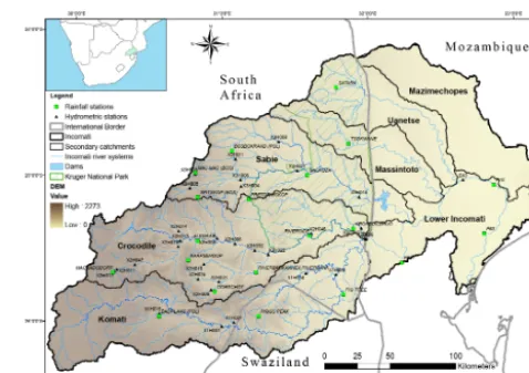
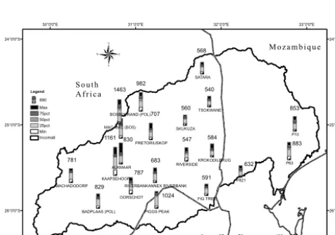
Figure 1. Map of the location of the study area, illustrating the main
sub-catchments, the hydrometric and rainfall stations analysed, and the basin topography and dams.
trends in streamflow and their possible linkages with the main drivers are analysed. Based on the findings, approaches and alternatives for improved water resource management and planning are proposed.
2 Methodology
2.1 Study area
The Incomati River basin is located in the south-eastern part of Africa and it is shared by the Kingdom of Swazi-land, the Republic of Mozambique and the Republic of South Africa (Fig. 1). The total basin area is approxi-mately 46 750 km2, of which 2560 km2(5.5 %) are in Swazi-land, 15 510 km2 (33.2 %) in Mozambique and 28 681 km2 (61.3 %) in South Africa. The Incomati watercourse includes the Komati, Crocodile, Sabie, Massintoto, Uanetse and Maz-imechopes rivers and the estuary. The Komati, Crocodile and Sabie are the main sub-catchments, contributing about 94 % of the natural discharge, with an area of 61 % of the basin. The Incomati River rises in the Highveld and escarpment (2000 m above sea level) in the west of the basin and drops to the coastal plain in Mozambique. The general climate in the Incomati River basin varies from a warm to hot humid climate in Mozambique to a cooler dry climate in South Africa in the west. The mean annual precipitation of about 740 mm a−1falls entirely during the summer months (Octo-ber to March). The Incomati (Fig. 1) can be topographically and climatically divided into three areas (TPTC, 2010):
– high escarpment, with a high rainfall (800 to 1600
Table 1. Summary of estimated natural streamflow, water demands in the Incomati basin in 106m3per year (TPTC, 2010) and major dams (>106m3)(Van der Zaag and Vaz, 2003).
Natural MAR First priority supplies Irrigation supplies Afforestration Total water use
Komati 1332 141.5 621 117 879.5
Crocodile 1124 74.7 482 158 714.7
Sabie 668 30 98 90 218
Massintoto 41 0.3 0 0 0.3
Uanetse 33 0.3 0 0 0.3
Mazimechopes 20 0 0 0 0
Lower Incomati 258 1.5 412.8 0 414.3
Mozambique 325 412.8
South Africa 2663 961
Swaziland 488 240
Total 3476 248 1614 365 2227
Tributary Country Major dam Year commissioned Storage capacity (106m3)
Komati South Africa Nooitgedacht 1962 81
Komati South Africa Vygeboom 1971 84
Komati Swaziland Maguga 2002 332
Komati Swaziland Sand River 1966 49
Lomati South Africa Driekoppies 1998 251
Crocodile South Africa Kwena 1984 155
Crocodile South Africa Witklip 1979 12
Crocodile South Africa Klipkopje 1979 12
Sabie South Africa Da Gama 1979 14
Sabie South Africa Injaka 2001 120
Sabie Mozambique Corumana 1988 879
Total 1989
* First priority supplies include domestic and industrial uses.
– Highveld and middle Lowveld, which lie between the
Drakensberg and the Lebombo Mountains, warmer than the escarpment (mean annual average of 14 to 22◦C), with rainfall that decreases towards the east (400 to 800 mm a−1) and high potential evaporation (2000 to 2200 mm a−1);
– coastal plain, located mostly in Mozambique, with
higher temperatures (mean annual average of 20 to 26◦C) and lower rainfall (400 to 800 mm a−1)in the west, increasing eastward towards the coast, where there is also high potential evaporation (2200 to 2400 mm a−1).
The geology is complex, characterised by sedimentary, vol-canic, granitic and dolomitic rocks, as well as Quaternary and recent deposits (Van der Zaag and Vaz, 2003). The soils in the basin are highly variable, ranging from moderately deep clayey loam in the west, to moderately deep sandy loam in the central areas and moderately deep clayey soils in the east. The dominant land uses in the catchment are commercial for-est plantations of exotic trees (pine, eucalyptus) in the es-carpment region, dryland crops (maize) and grazing in the Highveld region, and irrigated agriculture (sugarcane, veg-etables and citrus) in the Lowveld (DWAF, 2009b; Riddell et al., 2013). In the Mozambican coastal plains, sugarcane
and subsistence farming dominate. A substantial part of the basin has been declared a conservation area, which includes the recently established Greater Limpopo Transfrontier Park (the Kruger National Park in South Africa and the Limpopo National Park in Mozambique are part of it) (TPTC, 2010).
Table 2. Land-use and water-use change from the 1950s to 2004 in the Komati, Crocodile and Sabie sub-catchments. Source: adapted from
TPTC (2010).
1950s 1970s 1996 2004
Irrigation area (km2) 17.6 144.1 385.1 512.4
Afforested area (km2) 247 377 661 801
Domestic water use (106m3a−1) 0.5 7.7 15.5 19.7
Komati Industrial and mining water use (106m3a−1) 0 0 0.5 0.5
Water transfers out (106m3a−1):
To power stations in South Africa 3.4 103 98.1 104.7
To irrigation in Swaziland outside Komati 0 111.8 122.2 121.8
Irrigation area (km2) 92.8 365.8 427 510.7
Crocodile Afforested area (km2) 375 1550 1811 1941
Domestic water use (106m3a−1) 3 12.2 33.6 52.4
Industrial and mining water use (106m3a−1) 0.1 7.5 19.8 22.3
Irrigation area (km2) 27.7 68.4 113.4 127.6
Sabie Afforested area (km2) 428 729 708 853
Domestic water use (106m3a−1) 2.4 5.3 13 26.7
Industrial and mining water use (106m3a−1) 0 0 0 0
2.2 Data and analysis
2.2.1 Rainfall
Annual, monthly and daily rainfall data for southern Africa for the period of 1905 to 2000 were extracted from the Lynch (2003) database. The database consists of daily pre-cipitation records for over 12 000 stations in southern Africa, and data quality was checked and some data were patched. The main custodians of rainfall data are SAWS (South African Weather Service), SASRI (South Africa Sugarcane Research Institute) and ISCW (Institute for Soil Climate and Water). About 20 stations out of 374 available for Inco-mati were selected for detailed analysis. The selection cri-teria were the quality of data, evaluated by the percentage of reliable data in the database, and the representative spatial coverage of the basin. Eight of the 20 stations’ time series were extended up to 2012, using new data collected from the SAWS.
The spatial and temporal heterogeneity in rainfall across the study area was characterised using statistical analysis and annual anomalies. The time series of annual and monthly rainfall from each station were subjected to the Spearman test in order to identify trends for the periods of 1950–2000 and 1950–2011. Two intersecting periods were chosen to eval-uate the consistency of the trends. Due to natural climatic variability, there are sequences of wetter and drier periods, so some trends appearing in a specific period might be ab-sent when a longer or shorter period is considered. The Pet-titt test (PetPet-titt, 1979) is used to detect abrupt changes in the time series. Potential change points divide the time series into two sub-series. Then, the significance of the change in the mean and variance of the two sub-series is evaluated byF
andt tests. Potential change points were evaluated with a 0.8 probability threshold and significance of change was as-sessed withF andttests at the 95 % confidence level (Zhang et al., 2008; Love et al., 2010). The annual and monthly time series were also analysed for the presence of serial corre-lation. Tests were carried out using SPELL-stat v.1.5.1.0B (Guzman and Chu, 2003).
2.2.2 Streamflow
Stations
Incomati Developments Klipkopj
e Nooitge d acht W itklip Pr im ko p Vyge boom , Da Ga m a Mhl u me Tra n sf Kwe n a C o rrum ana Ngodwa na Drie koppie s Ma guga , In ya ka
Station Place 1959 1960 1961 1962 1963 1964 1965 1966 1967 1968 1969 1970 1971 1972 1973 1974 1975 1976 1977 1978 1979 1980 1981 1982 1983 1984 1985 1986 1987 1988 1989 1990 1991 1992 1993 1994 1995 1996 1997 1998 1999 2000 2001 2002 2003 2004 2005 2006 2007 2008 2009 2010 2011 2012
X1H001 Komati River @ Hooggenoeg N V
X1H003 Komati River @ Tonga N V M M
X1H014 Mlumati River @ Lomati D
X1H016 Buffelspruit @ Doornpoort X1H021 Mtsoli River @ Diepgezet
X2H005 Nels River @ Boschrand W
X2H006 Krokodil River @ Karino K W P K X2H008 Queens River @ Sassenheim
X2H010 Noordkaap River @ Bellevue X2H011 Elands River @ Geluk X2H012 Dawsons Spruit @ Geluk
X2H013 Krokodil River @ Montrose K X2H014 Houtbosloop @ Sudwalaskraal
X2H015 Elands River @ Lindenau
X2H016 Krokodil River @ Tenbosch K P K X2H022 Kaap River @ Dolton
X2H024 Suidkaap River @ Glenthorpe X2H031 Suidkaap River @ Bornmans Drift
X2H032 Krokodil River @ Weltevrede K WP K
X2H036 Komati River @ Komatipoort K P K M X2H046 Krokodil River @ Riverside K P K
X2H047 Swartkoppiesspruit @ Kindergoed X3H001 Sabie River @ Sabie X3H002 Klein Sabie River @ Sabie X3H003 Mac‐Mac River @ Geelhoutboom
X3H004 Noordsand River @ De Rust D X3H006 Sabie River @ Perry's Farm
X3H008 Sand River @ Exeter
X3H011 Marite River @ Injaka I
X3H015 Sabie River @ Lower Sabie Rest Camp D I X3H021 Sabie River @ Kruger Gate D I E23 Incomati River @ Ressano Garcia
E43 Incomati River @ Magude
[image:5.612.64.533.70.324.2]Good continuous data Missing data/no data Major data gaps/gauge limit
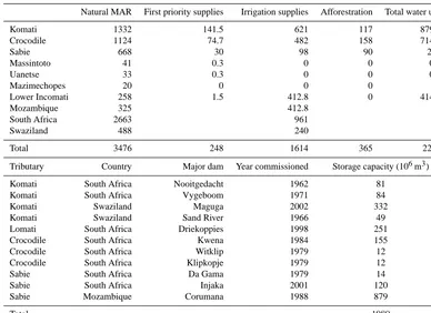
Figure 2. Streamflow data used on this study, with indication of time series length, data quality, and missing data. Major developments in
the basin, such as dams, are on the top horizontal line in the year they were commissioned; indication is made of the gauges affected by the developments by the initial letter of the dam.
2.2.3 Indicators of hydrologic alteration
The US Nature Conservancy developed a statistical software program known as the Indicators of Hydrologic Alteration (IHA) for assessing the degree to which human activities have changed flow regimes. The IHA method (Richter et al., 1996, 2003; Richter and Thomas, 2007) is based upon the concept that hydrologic regimes can be characterised by five ecologically relevant attributes, listed in Table 4: (1) mag-nitude of monthly flow conditions; (2) magmag-nitude and dura-tion of extreme flow events (e.g. high and low flows); (3) the timing of extreme flow events; (4) frequency and duration of high low flow pulses; and (5) the rate and frequency of changes in flows. It consists of 67 parameters, which are subdivided into two groups – 33 IHA parameters and 34 en-vironmental flow component parameters. These hydrologic parameters were developed based on their ecological rele-vance and their ability to reflect human-induced changes in flow regimes across a broad range of influences including dam operations, water diversions, groundwater pumping, and landscape modification (Mathews and Richter, 2007). 33 se-lected gauges from the Incomati basin were analysed with this method using daily flow data. Many studies successfully applied the methodology of Indicators of Hydrologic Alter-ation, in order to assess impacts on streamflow caused by an-thropogenic drivers (Maingi and Marsh, 2002; Taylor et al., 2003; Mathews and Richter, 2007; De Winnaar and Jewitt,
2010; Masih et al., 2011). In the case of the present study, the indicators of the magnitude of monthly flow, the magnitude and duration of extreme flow, as well as timing, were anal-ysed for the period 1970–2011, to assess whether consistent trends of increase or decrease of the hydrological indicators were present.
The IHA software was used to identify trends of the streamflow time series, based on the regression of least squares. This trend is evaluated with theP value, and only trends withP ≤0.05 were considered significant trends, the value of the slope of the trend line indicating an increas-ing or decreasincreas-ing trend. This information was compiled and mapped for the various hydrological indicators using Ar-cGIS 9.3.
2.2.4 Land-use analysis
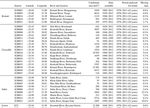
Table 3. Hydrometric stations analysed, location, catchment area, data length and missing data.
Catchment Data Period analysed Missing Station Latitude Longitude River and location area (km2) available for trends data X1H001 −26.04 31.00 Komati River, Hooggenoeg 5499 1909–2012 1970–2011 (42 years) 8.0 % X1H003 −25.68 31.78 Komati River, Tonga 8614 1939–2012 1970–2011 (42 years) 6.8 % Komati X1H014 −25.67 31.58 Mlumati River, Lomati 1119 1968–2012 1978–2011 (34 years) 0.5 % X1H016 −25.95 30.57 Buffelspruit, Doornpoort 581 1970–2012 1970–2011 (42 years) 3.4 % X1H021 −26.01 31.08 Mtsoli River, Diepgezet 295 1975–2012 1976–2011 (36 years) 2.7 % X2H005 −25.43 30.97 Nels River, Boschrand 642 1929–2012 1970–2011 (42 years) 0.8 % X2H006 −25.47 31.09 Krokodil River, Karino 5097 1929–2012 1970–2011 (42 years) 0.1 % X2H008 −25.79 30.92 Queens River, Sassenheim 180 1948–2012 1970–2011 (42 years) 0.5 % X2H010 −25.61 30.87 Noordkaap River, Bellevue 126 1948–2012 1970–2011 (42 years) 5.7 % X2H011 −25.65 30.28 Elands River, Geluk 402 1956–1999 1957–1999 (43 years) 0.9 % X2H012 −25.66 30.26 Dawsons Spruit, Geluk 91 1956–2012 1970–2011 (42 years) 0.3 % X2H013 −25.45 30.71 Krokodil River, Montrose 1518 1959–2012 1970–2011 (42 years) 1.6 % X2H014 −25.38 30.70 Houtbosloop, Sudwalaskraal 250 1958–2012 1970–2011 (42 years) 5.1 % Crocodile X2H015 −25.49 30.70 Elands River, Lindenau 1554 1959–2012 1970–2011 (42 years) 3.1 % X2H016 −25.36 31.96 Krokodil River, Tenbosch 10 365 1960–2012 1970–2011 (42 years) 5.6 % X2H022 −25.54 31.32 Kaap River, Dolton 1639 1960–2012 1970–2011 (42 years) 5.7 % X2H024 −25.71 30.84 Suidkaap River, Glenthorpe 80 1964–2012 1970–2011 (42 years) 1.7 % X2H031 −25.73 30.98 Suidkaap River, Bornmans Drift 262 1966–2012 1966–2011 (46 years) 5.0 % X2H032 −25.51 31.22 Krokodil River, Weltevrede 5397 1968–2012 1970–2011 (42 years) 2.4 % X2H036 −25.44 31.98 Komati River, Komatipoort 21 481 1982–2012 1983–2011 (28 years) 4.1 % X2H046 −25.40 31.61 Krokodil River, Riverside 8473 1985–2012 1986–2011 (26 years) 2.0 % X2H047 −25.61 30.40 Swartkoppiesspruit, Kindergoed 110 1985–2012 1986–2011 (26 years) 2.2 % X3H001 −25.09 30.78 Sabie River, Sabie 174 1948–2012 1970–2011 (42 years) 0.8 % X3H002 −25.09 30.78 Klein Sabie River, Sabie 55 1963–2012 1970–2011 (42 years) 0.4 % X3H003 −24.99 30.81 Mac-Mac River, Geelhoutboom 52 1948–2012 1970–2011 (42 years) 0.5 % X3H004 −25.08 31.13 Noordsand River, De Rust 200 1948–2012 1970–2011 (42 years) 3.9 % Sabie X3H006 −25.03 31.13 Sabie River, Perry’s Farm 766 1958–2000 1970–1999 (30 years) 2.6 % X3H008 −24.77 31.39 Sand River, Exeter 1064 1967–2011 1968–2011 (43 years) 15.5 % X3H011 −24.89 31.09 Marite River, Injaka 212 1978–2012 1979–2011 (32 years) 7.6 % X3H015 −25.15 31.94 Sabie River, Lower Sabie Rest Camp 5714 1986–2012 1988–2011 (24 years) 8.2 % X3H021 −24.97 31.52 Sabie River, Kruger Gate 2407 1990–2012 1991–2011 (21 years) 10.8 % Lower E23 −25.44 31.99 Incomati River, Ressano Garcia 21 200 1948–2011 1970–2011 (42 years) 9.0 % Incomati E43 −25.03 32.65 Incomati River, Magude 37 500 1952–2011 1970–2011 (42 years) 3.5 %
Table 4. Hydrologic parameters used in the range of variability approach (Richter et al., 1996).
Indicators of hydrologic Regime Hydrological
alteration group characteristics parameters
Group 1: magnitude of monthly water conditions
Magnitude timing Mean value for each calendar month
Group 2: magnitude and duration of annual extreme water conditions
Magnitude duration Annual minima and maxima based on
1, 3, 7, 30 and 90 day means
Group 3: timing of annual extreme water conditions
Timing Julian date of each annual 1 day
maximum and minimum
Group 4: frequency and duration of high/low pulses
Frequency and duration No. of high and low pulses each year
Mean duration of high and low pulses within each year (days)
Group 5: rate/frequency of water condition changes
Rates of change of frequency
Means of all positive and negative differences between consecutive daily values
[image:6.612.87.506.474.687.2]Table 5. Description of rainfall stations analysed for trends, the long-term mean annual precipitation (MAP) in mm a−1, the standard vari-ation, and the detection of the trend (confidence level of 95 % using the Spearman test) and occurrence change point (using the Pettitt test followed by theT test of stability of the mean and theFtest of the stability of variance).
Analysis for the period 1950 to 2011
Station Altitude MAP Preliable Mean SD Trend
Name ID Latitude Longitude (m a.s.l.) (mm) (%) (mm a−1) (mm a−1) Spearman Pettitt Machadodorp 0517430 W −25.67 30.25 1563 781 79.6 773 134
Badplaas (Pol) 0518088 W −-25.97 30.57 1165 829 90.6 817 153
Kaapsehoop 0518455 W −25.58 30.77 1564 1443 78.5 1461 286 Decr (1975)
Mac-Mac (Bos) 0594539 W −24.98 30.82 1295 1463 75.1 1501 287
Spitskop (Bos) 0555579 W −25.15 30.83 1395 1161 68.5 1197 266 Decr Decr (1978)*
Alkmaar 0555567 W −25.45 30.83 715 830 95.2 874 172
Oorschot 0518859 W −25.80 30.95 796 787 92.2 775 185
Bosbokrand (Pol) 0595110 W −24.83 31.07 778 982 82.4 919 297 Decr (1978)* Pretoriuskop 0556460 W −25.17 31.18 625 707 60.0 734 188
Riverbank 0519310 W −25.67 31.23 583 683 70.5 782 163 Incr Incr (1977)** Piggs Pig 0519448 A −25.97 31.25 1029 1024 40.1 1075 315 Decr Decr (1978)*
Skukuza 0596179 W −25.00 31.58 300 560 63.1 566 140
Riverside 0557115 W −25.42 31.60 315 547 66.5 520 187
[image:7.612.58.536.117.343.2]Satara 0639504 W −24.40 31.78 257 568 42.1 602 151 Incr Incr (1971)
Fig Tree 0520589 W −25.82 31.83 256 591 63.4 594 145 Decr Decr (1978)*
Tsokwane 0596647 W −24.78 31.87 262 540 66.1 544 134 Incr (1971)*
Krokodilbrug 0557712 W −25.37 31.90 192 584 62.9 590 147
Moamba P821 M −25.60 32.23 108 632 63.9 633 185
Xinavane P10 M −25.07 32.87 18 853 76.2 773 241
Manhica P63 M −25.40 32.80 33 883 86.2 903 275 Incr (1970)**
* Significant change with 2.5 % significance level withTtest of stability of mean. ** Significant change with 2.5 % significance level withTtest of stability of mean andFTest of stability of variance. Explanatory note: MAP is the mean annual precipitation, and P reliable is the percentage of reliable data for the rainfall station, as assessed by Lynch (2003) for the period 1905 to 1999. The mean refers to the average of the total annual precipitation for the period of 1950 to 2011. In the trend Spearman column, only stations that had trends significant at the 95 % confidence level are indicated with Decr or Incr, corresponding to a decreasing or increasing trend, respectively. In the Pettitt column, the direction of change and year are indicated, as well as the significance of the change point.
568
540 982
560 853
707
584
883 547
830
632 683
781
787 591
829 1463
1161
1024
P10
P63
P821 SATARA
SKUKUZA
ALKMAAR
TSOKWANE
OORSCHOT FIG TREE
RIVERSIDE
KAAPSEHOOP
PIGGS PEAK MACHADODORP
PRETORIUSKOP
KROKODILBRUG MAC MAC (BOS)
BADPLAAS (POL) BOSBOKRAND (POL)
RIVERBANKANNEX RIVERBANK
33°0'0"E 33°0'0"E
32°0'0"E 32°0'0"E
31°0'0"E 31°0'0"E
30°0'0"E 30°0'0"E
24°0'0"S 24°0'0"S
25°0'0"S 25°0'0"S
26°0'0"S 26°0'0"S
Legend 690 Max 75pct 50pct 25pct Min Incomati
®
0 25 50 100
Kilometers
Mozambique
Swaziland South
Africa
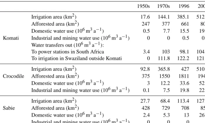
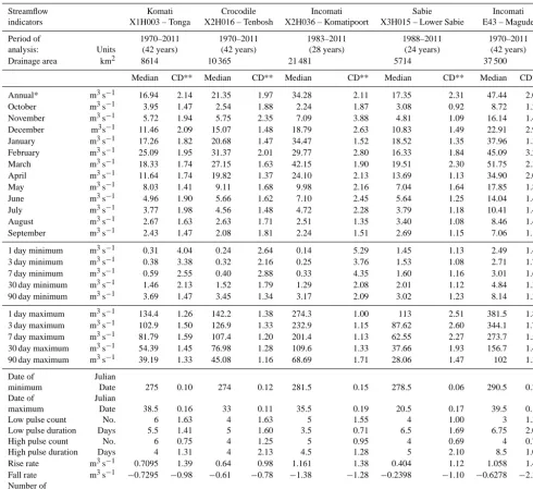
Figure 3. Map illustrating the spatial variation of annual rainfall
across the Incomati basin (minimum, 25 %, median, 75 %, and max-imum annual precipitation are shown in the bar; the number on top of the bar is the Mean Annual Precipitation for the period 1950– 2000).
3 Results
3.1 Rainfall
Data series of 20 rainfall stations were statistically analysed for the period 1950–2011 (Table 5). The variability of rain-fall across the basin was confirmed to be high, both intra-and inter-annually, with a wide range between years. This variability is highest for the stations located in mountainous areas. The variability across the basin is also significant, as illustrated by the boxplot of Fig. 3.
The Spearman trend test revealed that only 5 of the 20 in-vestigated stations showed significant trends of increase (2 stations) and decrease (3 stations). However, the stations that presented significant trends are also stations with a lower per-centage of reliability; thus, it is possible that the trend identi-fied could be affected by data infilling procedures. There was no serial correlation of annual and monthly time series. Some change points were identified using the Pettitt test, mostly in the years 1971 and 1978 (Table 5). Only 2 stations out of the 20 studied showed significant change towards a wetter regime (Riverbank and Manhica).
[image:7.612.48.286.401.568.2]Table 6. Hydrological indicators of main sub-catchments.
Streamflow Komati Crocodile Incomati Sabie Incomati
indicators X1H003 – Tonga X2H016 – Tenbosh X2H036 – Komatipoort X3H015 – Lower Sabie E43 – Magude
Period of 1970–2011 1970–2011 1983–2011 1988–2011 1970–2011
analysis: Units (42 years) (42 years) (28 years) (24 years) (42 years)
Drainage area km2 8614 10 365 21 481 5714 37 500
Median CD** Median CD** Median CD** Median CD** Median CD**
Annual* m3s−1 16.94 2.14 21.35 1.97 34.28 2.11 17.35 2.31 47.44 2.01
October m3s−1 3.95 1.47 2.54 1.88 2.24 1.87 3.08 0.92 8.72 1.21
November m3s−1 5.72 1.94 5.75 2.35 7.09 3.88 4.81 1.09 16.14 1.49
December m3s−1 11.46 2.09 15.07 1.48 18.79 2.63 10.83 1.49 22.91 2.90
January m3s−1 17.26 1.82 20.68 1.47 34.47 1.52 18.52 1.35 37.96 1.35
February m3s−1 25.09 1.95 31.37 2.01 29.77 2.80 16.33 1.84 45.09 3.21
March m3s−1 18.33 1.74 27.15 1.63 42.15 1.90 19.51 2.30 51.75 2.32
April m3s−1 11.64 1.74 19.82 1.37 24.10 2.13 13.69 1.13 34.90 2.03
May m3s−1 8.03 1.41 9.11 1.68 9.98 2.16 7.04 1.64 17.85 1.86
June m3s−1 4.96 1.90 5.66 1.62 7.10 2.45 5.64 1.25 14.04 1.44
July m3s−1 3.77 1.98 4.56 1.48 4.72 2.28 3.79 1.18 10.41 1.47
August m3s−1 2.67 1.63 2.63 1.71 2.51 1.35 3.40 1.08 8.46 1.41
September m3s−1 2.43 1.47 2.08 1.81 2.24 1.51 2.69 1.15 7.06 1.11
1 day minimum m3s−1 0.31 4.04 0.24 2.64 0.14 5.29 1.45 1.13 2.49 1.48 3 day minimum m3s−1 0.38 3.38 0.32 2.16 0.25 3.76 1.53 1.08 2.71 1.76 7 day minimum m3s−1 0.59 2.55 0.40 2.88 0.33 4.35 1.60 1.16 3.01 1.61 30 day minimum m3s−1 1.46 2.13 1.52 1.79 1.29 2.08 2.01 1.12 4.84 1.37 90 day minimum m3s−1 3.69 1.47 3.45 1.34 3.17 2.09 3.02 1.23 8.14 1.38 1 day maximum m3s−1 134.4 1.26 142.2 1.38 274.3 1.00 113 2.51 381.5 1.80 3 day maximum m3s−1 102.9 1.50 126.9 1.33 232.9 1.15 87.62 2.60 344.1 1.74 7 day maximum m3s−1 81.79 1.59 107.4 1.20 201.4 1.13 62.55 2.27 273.7 1.56 30 day maximum m3s−1 54.39 1.45 76.98 1.28 109.6 1.33 37.66 1.93 156.7 1.45 90 day maximum m3s−1 39.19 1.33 45.08 1.16 68.69 1.71 28.06 1.47 102 1.32
Date of Julian
minimum Date 275 0.10 274 0.12 281.5 0.15 278.5 0.06 290.5 0.21
Date of Julian
maximum Date 38.5 0.16 33 0.11 35.5 0.19 20.5 0.17 39.5 0.14
Low pulse count No. 6 1.63 4 1.63 5 1.55 4 1.00 3 1.33
Low pulse duration Days 5.5 1.41 5 1.60 3.5 0.71 6.5 1.69 6.75 2.09
High pulse count No. 6 0.75 4 1.25 5 0.95 4 0.69 4 0.75
High pulse duration Days 4 1.31 4 2.13 4.5 1.28 5 2.10 8.5 1.03
Rise rate m3s−1 0.7095 1.39 0.64 0.98 1.161 1.38 0.404 1.12 1.058 1.43 Fall rate m3s−1 −0.7295 −0.98 −0.61 −0.78 −1.38 −1.28 −0.2398 −1.10 −0.6278 −2.31 Number of
reversals No 111.5 0.26 113 0.42 121 0.18 95 0.29 86 0.49
* In the annual statistics, the mean and coefficient of variation were used. **CD is the coefficient of dispersion. More details about CD are available in the text.
Mussá et al. (2013) studied the trends of annual and dry extreme rainfall using the Standardized Precipitation Index (SPI), and also found no significant trends in annual rainfall extremes across the Crocodile sub-catchment.
3.2 Variability of streamflow
The metrics of the different hydrologic indicators were com-piled as an output of the IHA analysis, which is illustrated for the gauging stations located at the outlet (or the most down-stream) of each main sub-catchment in Table 6. The variabil-ity is described, using non-parametric statistics (median and coefficient of dispersion), because the hydrological time
se-ries are not normally distributed, but are positively skewed. The coefficient of dispersion (CD) is defined as CD=(75th percentile – 25th percentile)/50th percentile. The larger the CD, the larger the variation of the parameter will be.
The flow patterns are consistent with the summer rainfall regime, with the highest flow and rainfall events associated with tropical cyclone activity in January–March.
0.0 1.0 2.0 3.0 4.0 5.0 6.0 7.0 8.0 9.0 10.0
October November December January February March April May June July August September
M
ed
ia
n S
tre
amf
lo
w
[mm p
er
mo
nt
h]
[image:9.612.310.545.62.225.2]KOMATI X1H003 - TONGA CROCODILE X2H016 - TENBOSH SABIE X3H015 - LOWER SABIE INCOMATI E43 - MAGUDE
Figure 4. Median of observed daily streamflow for the gauges
lo-cated at the outlets of the major sub-catchments: Komati, Crocodile, Lower Sabie and Incomati (based on daily time series from 1970 to 2011).
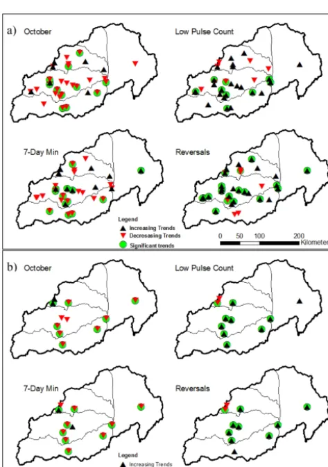
Figure 5. Trends of different indicators of streamflow: (a) for period
1970–2011; (b) for period 1950–2011.
(Hughes and Mallory, 2008; DWAF, 2009a), which are more intense in the Komati and Crocodile sub-catchments.
[image:9.612.49.287.67.159.2]Another aspect to note is that the flows of February are likely to be higher than observed records, but high stream-flow extremes are not fully captured by the current monitor-ing network, due to gauge limits.
Figure 6. Count of significant trends. Declining trends are in red
and increasing trends in green. The size of the pie is proportional to the total number of significant trends.
3.3 Trends in streamflow
Figure 5 presents a spatial plot of trends for selected hydro-logical indicators for the periods 1970–2011 (Fig. 5a) and 1950–2011 (Fig. 5b). The significant trends are highlighted with a circle. Table 7 presents the slope of the trend lines andP values for the gauges located at the outlet, or the most downstream point of each main sub-catchment. There is a significant trend of decreasing mean flow in October at al-most all stations, especially the ones located on the main stem of the Crocodile and Komati rivers. October is the month of the start of the rainy season, when the dam levels are lowest and irrigation water requirements highest (DWAF, 2009a; ICMA, 2010).
This trend is consistent with the decreasing trends of min-imum flows, as exemplified by the 7 day minmin-imum. In con-trast, it can be seen that the count of low pulses increased significantly in many gauges, which indicates the more fre-quent occurrence of low flows. Another striking trend is the significant increase in the number of reversals at almost all stations. Reversals are calculated by dividing the hydrologic record into “rising” and “falling” periods, which correspond to periods in which daily changes in flows are either positive or negative, respectively. The number of reversals is the num-ber of times that the flow switches from one type of period to another. The observed increased number of reversals is likely due to the effect of flow regulation and water abstractions.
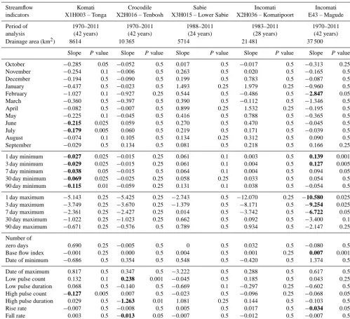
[image:9.612.50.287.246.582.2]Table 7. Trends of the hydrological indicators for the period 1970–2011. In bold are significant trends at the 95 % confidence level.
Streamflow Komati Crocodile Sabie Incomati Incomati
indicators X1H003 – Tonga X2H016 – Tenbosh X3H015 – Lower Sabie X2H036 – Komatipoort E43 – Magude
Period of 1970–2011 1970–2011 1988–2011 1983–2011 1970–2011
analysis (42 years) (42 years) (24 years) (28 years) (42 years)
Drainage area (km2) 8614 10 365 5714 21 481 37 500
Slope Pvalue Slope Pvalue Slope Pvalue Slope Pvalue Slope Pvalue
October −0.285 0.05 −0.052 0.5 0.017 0.5 −0.017 0.5 −0.313 0.25
November −0.254 0.1 −0.006 0.5 0.263 0.5 0.020 0.5 −0.165 0.5
December −0.194 0.5 −0.090 0.5 0.199 0.5 0.783 0.5 −0.087 0.5
January −0.437 0.5 −0.023 0.5 1.493 0.25 1.979 0.25 −0.960 0.5
February −1.027 0.1 −0.927 0.25 0.544 0.5 −0.486 0.5 −2.847 0.05
March −0.360 0.5 −0.397 0.5 0.390 0.5 −0.112 0.5 −1.346 0.5
April −0.082 0.5 −0.007 0.5 0.899 0.25 1.532 0.25 −0.195 0.5
May −0.225 0.1 −0.045 0.5 0.416 0.5 0.788 0.5 −0.365 0.5
June −0.215 0.025 0.059 0.5 0.270 0.5 0.470 0.5 −0.045 0.5
July −0.179 0.005 0.060 0.5 0.219 0.5 0.171 0.5 −0.039 0.5
August −0.074 0.1 0.105 0.5 0.134 0.25 0.312 0.5 0.090 0.5
September −0.029 0.5 0.134 0.5 0.081 0.5 0.218 0.5 0.166 0.25
1 day minimum −0.027 0.025 −0.015 0.25 0.061 0.1 0.003 0.5 0.139 0.001
3 day minimum −0.029 0.025 −0.015 0.25 0.061 0.1 0.004 0.5 0.127 0.005
7 day minimum −0.038 0.05 −0.015 0.5 0.064 0.1 0.004 0.5 0.094 0.05
30 day minimum −0.069 0.025 −0.025 0.25 0.058 0.25 0.033 0.5 0.054 0.5
90 day minimum −0.115 0.01 −0.059 0.25 0.131 0.1 0.038 0.5 −0.054 0.5
1 day maximum −5.143 0.25 −5.425 0.25 −2.743 0.5 −12.070 0.25 −10.580 0.025
3 day maximum −3.749 0.25 −3.670 0.25 −1.379 0.5 −8.171 0.5 −9.254 0.025
7 day maximum −2.361 0.25 −2.427 0.25 0.014 0.5 −3.742 0.5 −6.722 0.05
30 day maximum −1.022 0.25 −1.023 0.25 0.662 0.5 0.092 0.5 −3.400 0.1
90 day maximum −0.671 0.25 −0.576 0.5 0.789 0.5 0.934 0.5 −2.147 0.25
Number of
zero days 0.690 0.25 −0.005 0.5 0 0.5 0.032 0.5 −0.080 0.5
Base flow index −0.001 0.25 0.000 0.5 0.004 0.5 0.001 0.25 0.007 0.001
Date of minimum −0.686 0.5 0.354 0.5 0.548 0.5 −0.420 0.5 1.374 0.5
Date of maximum 0.817 0.5 0.347 0.5 −3.222 0.5 0.288 0.5 0.617 0.5
Low pulse count 0.132 0.1 0.238 0.001 −0.045 0.5 0.185 0.5 0.043 0.25
Low pulse duration 0.068 0.5 −0.140 0.5 −0.669 0.1 −0.297 0.25 −0.602 0.5
High pulse count −0.127 0.005 0.007 0.5 −0.023 0.5 −0.096 0.25 −0.068 0.05
High pulse duration 0.029 0.5 −1.263 0.01 1.081 0.25 0.144 0.5 −0.103 0.5
Rise rate −0.007 0.5 −0.008 0.5 0.005 0.5 0.017 0.5 −0.034 0.05
Fall rate 0.003 0.5 −0.013 0.05 −0.007 0.5 −0.012 0.5 −0.007 0.5
Number of reversals 0.574 0.1 1.083 0.01 0.723 0.5 0.560 0.5 0.764 0.005
The cross-compensation can also be observed on a basin scale in the Sabie, where the trends of decreasing flows are not so frequent or significant. It is likely that this occurs be-cause the majority of the Sabie falls under the conservation area of the Kruger National Park (KNP), and therefore fewer abstractions occur compared to other sub-catchments, as il-lustrated in Table 1. The KNP has been playing an important role in the catchment management fora set up by the Inko-mati Catchment Management Agency (ICMA), which con-cern the provision of environmental minimum flows, in order to maintain ecosystem services and biodiversity in the park (Pollard et al., 2012; Riddell et al., 2013).
Table 7 illustrates that many of the trends observed in the Sabie sub-catchment contrast with those observed in the Komati and Crocodile sub-catchments. Thus, the trends ob-served in downstream Magude (station E43) in Mozambique are the result of a combination of the positive effect of the conservation approach of KNP on the Sabie, and the negative effect of flow reductions on the Crocodile and the Komati.
tribu-Figure 7. Land-use land-cover map of Incomati (ICMA, 2010; TPTC, 2010) and streamflow trends in the month of October.
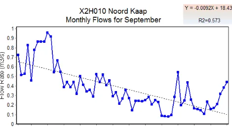
Figure 8. Plot of median monthly flows for September for the entire
time series (1949–2011) on the Noord Kaap gauge, located in the Crocodile sub-catchment.
taries both have significant decreasing trends of their mean monthly flows, as well as the low flows; the Kwena Dam, lo-cated on the main stem of the Crocodile, on the other hand, is managed in a way so as to augment the flows during the dry season.
It is important to note that these trends are even more pro-nounced when longer time series are considered. Two exam-ples from the Crocodile basin are presented below.
3.3.1 Example of decreasing trends: Noord Kaap X2H010
[image:11.612.52.287.395.524.2]0 0.2 0.4 0.6 0.8 1 1.2 1.4
M
ed
ia
n
Fl
ow
s m
3/s
X2H010 Noord Kaap Monthly Flow Alteration (1949-2011)
[image:12.612.52.280.65.219.2]Pre-impact period: 1949-1974 Post-impact period: 1978-2011
Figure 9. Plot of median monthly flows for two periods (1949–1974
and 1978–2011) on the Noord Kaap gauge, located in the Crocodile sub-catchment.
streamflow reduction activity (SFRA) (Jewitt, 2002, 2006b). A recent study by van Eekelen et al. (2015) finds that stream-flow reduction due to forest plantations may be 2 or even 3 times more than that allowed by the Interim IncoMaputo Agreement.
3.3.2 Impact of the Kwena Dam on streamflows of the Crocodile River
The Kwena Dam is the main reservoir in the Crocodile sys-tem, located upstream in the catchment and commissioned in 1984. The dam is used to improve the assurance of supply of water for irrigation purposes in the catchment. The Montrose gauge (X2H013) is located a few kilometres downstream of this dam. The two-period (1959–1984 and 1986–2011) anal-ysis illustrates the main impacts of the Kwena Dam on the river flow regime, namely the dampening of peak flows and an increase in low flows (Fig. 10). These results are con-sistent with the analysis conducted by Riddell et al. (2013), which found significant alterations of the natural flow regime in the Crocodile basin over the past 40 years. Similar impacts were found in studies in different parts of the world (Richter et al., 1998; Bunn and Arthington, 2002; Maingi and Marsh, 2002; Birkel et al., 2014).
It can be seen that this reservoir is managed to augment the low flows and attenuate floods. This change in the flow regime influences the streamflow along the main stem of the Crocodile River, but as tributaries join and water is ab-stracted, the effect is reduced. At the outlet at Tenbosch gauge X2H016 (Fig. 6 and Table 7), the effects of flow regu-lation and water abstractions have counter-balanced the con-trasting trends observed upstream.
3.3.3 Impact of anthropogenic actions
As can be seen from water-use information, the impacts of land-use change and water abstractions are the main drivers
0 1 2 3 4 5 6 7 8 9 10
M
ed
ian
F
lo
w
s (
m
3/s
)
X2H013 Montrose Monthly Flow Alteration (1959-2011)
Pre-impact period: 1959-1984 Post-impact period: 1986-2011
Figure 10. Impact of the Kwena Dam (commissioned in 1984) on
streamflows of the Crocodile River, Montrose gauge X2H013.
of changes in the flow regime on the Incomati. However, the situation is variable along the catchment. In the Sabie system, in spite of large areas of commercial forestry in the head-waters, the indicators of mean, annual and low flows do not show significant trends (Table 7). This can be explained by the fact that most of the forestry area was already established during the period of analysis (1970–2011) (DWAF, 2009c). The fact that a large proportion of the Sabie sub-catchment is under conservation land use (KNP and other game reserves) also plays an important role in maintaining the natural flow regime.
On the Crocodile, however, irrigated agriculture, forestry and urbanisation were the most important anthropogenic drivers. They affect the streamflow regime, the water quantity and possibly the water quality as well (beyond the scope of this analysis). This has important implications when environ-mental flow requirements and minimum cross-border flows need to be adhered to. Pollard and du Toit (2011a) and Rid-dell et al. (2013) have demonstrated that the Crocodile River is not complying with environmental flow requirements dur-ing most of the dry season at the outlet.
[image:12.612.312.542.67.219.2]4 Discussion
4.1 Limitations of this study
The available data series have some gaps, especially during high flow periods. Because of this, the analysis of high flow extremes is highly uncertain. For the trend analysis, the pe-riod of common data followed the construction of several im-poundments and other developments.
Another challenge is the disparity of data availability across the different riparian countries. In Mozambique, only two gauges had reliable flow data for this analysis, represent-ing the entire lower Incomati system. The rivers Massintoto, Uanetse and Mazimechopes in Mozambique do not have ac-tive flow gauges. There is definitely a need to strengthen the hydrometric monitoring network in the Mozambican part of the basin, as well as in the tributaries originating in the Kruger National Park.
4.2 What are the most striking trends and where do they occur?
The analysis resulted in the identification of major trends, including
– decreasing trends in the magnitude of monthly flow
(significant for low flow months, e.g. October), mini-mum flow (1, 3, 7, 30 and 90 day minima) and the oc-currence of high flow pulses,
– significant increasing trends of the magnitude of
monthly flow (August and September) in some loca-tions in the Crocodile and Sabie, and in the occurrence of flow reversals basin-wide, and
– Some gauges showed no significant change or no clear
pattern of change in the parameters analysed. These are mainly gauges located on the Sabie, which by 1970 had already established the current land use.
In the Komati system, the flow regulation and water abstrac-tions have strong impacts on streamflow. Most gauges are severely impacted and it is quite difficult to characterise natu-ral flow conditions. Flow regulation has the largest impact on low flow and minimum flows. In the Komati, irrigated agri-culture is significant, particularly sugarcane. The upstream dams of Nooitgedacht and Vygeboom are mainly used to supply cooling water to ESKOM power stations outside the basin; thus, this water is exported and not used within the basin.
In the Crocodile system, flow regulation by the Kwena Dam has attenuated extreme flow events. The high flows are reduced and the low flows generally increase, leading to reverse seasonality downstream. Reverse seasonality is the change in timing of hydrograph characteristics, for exam-ple, the occurrence of low flows in the wet season or high flows in the dry season. The Kwena Dam is used to improve
the assurance of the supply of water for irrigation purposes in the catchment. However, Noord Kaap gauge X2H010, a headwater tributary of the Crocodile system, experiences a significant and dramatic reduction in flows, shown in the monthly flow, and the low flow parameters. This change was compared with the increase in the area under forestry in the sub-catchment, as well as with the increase in irrigation. The comparison revealed that the land-use change was the main driver of the flow alteration.
In the Sabie system, most gauges did not show significant trends. This is most likely due to fewer disturbances com-pared to the other main catchments: lower water demands, fewer water abstractions and larger areas under conservation. During the period 1970–2011 there were no clear impacts of climatic change (in terms of rainfall) on streamflow.
4.3 Implications of these findings for water resource management
The results of this study illustrate some hotspots where more attention should be put in order to ensure provision of water to society and the environment. When the analysis of trends is combined with the land use of the basin (Fig. 7), it is clear that the majority of gauges with decreasing trends are lo-cated in areas where forestry or irrigated agriculture dom-inates the land use and where conservation approaches are less prevalent. The presence of water management infrastruc-ture (dams) greatly influences the flow regime.
For the management of water resources in the basin, it is important to note some clear patterns, illustrated by the Sa-bie, Crocodile and Komati. The Sabie flows generated in the upper parts of the catchment persist until the outlet, whilst in other rivers, flows are highly modified. This suggests that the use of the conservation approach through the strategic adap-tive management of the Kruger National Park (KNP) and the Inkomati Catchment Management Agency (ICMA), which are stronger on the Sabie, can be very beneficial for keeping environmental flows in the system. It is important to consider not only the magnitude of flows, but their duration and timing as well.
irreversible, including the social upheaval caused by the re-settlement of communities, loss of ecosystems and biodi-versity, increased sediment trapping, irreversible alteration of flow regimes and the prohibitive cost of decommission-ing (see, for an overview, Tullos et al., 2009, and Moore et al., 2010). It is therefore important to explore alternative op-tions fully before deciding on the construction of more large dams. So, alternative possibilities of restoring natural stream flows and/or increasing water storage capacity should be vestigated further and adopted. These alternatives could in-clude aquifer storage, artificial recharge, rainfall harvesting, decentralised storage, and reducing the water use of exist-ing uses and users, includexist-ing irrigation, industry and forest plantations. The operation rules of existing and future dams should also include objectives to better mimic crucial aspects of the system’s natural variability.
Given the likely expansion of water demands due to urban-isation and industrial development, it is also important that water demand management and water conservation measures are better implemented in the basin. For example, there could be systems to reward users that use technology to improve their water-use efficiency and municipalities that encourage their users to lower water use.
This study also shows the complexity of water resource availability and variability. The complexity is even more rel-evant, considering that this is a trans-boundary basin and that there are international agreements regarding minimum cross-border flows and maximum development levels that have to be adhered to (Nkomo and van der Zaag, 2004; Pollard and Toit, 2011a, b; Riddell et al., 2013).
There is a great discrepancy in data availability between different riparian countries. It is important that Mozambique, in particular, improves its monitoring network, in order better to assess the impact of various management activities occur-ring upstream on the state of water resources. The monitooccur-ring of hydrological extremes should receive more attention, with the focus on increasing the accuracy of recording the flood events. The improvement of the monitoring network can be achieved by various means, such as
– water management institutions collaborating more
in-tensely with academic and consultant institutions,
– developing realistic plans to improve monitoring and
data management,
– learning from other countries/institutions that have
ade-quate monitoring in place,
– using modern ICT and other technologies, which may
become cheaper and more accessible, and
– involving more stakeholders and citizens in data
collec-tion.
5 Conclusions
The research conducted reveals the dynamics of streamflow and their drivers in a river basin.
The statistical analysis of rainfall data revealed no consis-tent significant trend of increase or decrease for the studied period. The analysis of streamflow, on the other hand, re-vealed significant decreasing trends of streamflow indicators, particularly the median monthly flows of September and Oc-tober, and low flow indicators. This study concludes that land use and flow regulation are the largest drivers of streamflow trends in the basin. Indeed, over the past 40 years, the areas under commercial forestry and irrigated agriculture have in-creased over 4 times, increasing the consumptive water use basin-wide.
The study therefore recommends that the strategic adap-tive management adopted by the Kruger National Park and the Inkomati Catchment Management Agency should be employed further in the basin. Water demand management and water conservation should be alternative options to the development of dams, and should be investigated further and established in the basin. Land-use practices, particularly forestry and agriculture, have a significant impact on the wa-ter quantity of the basin; therefore, stakeholders from these sectors should work closely with the water management in-stitutions when planning for future developments and water allocation plans.
Considering the high spatial variability in the observed changes, no unified approach will work, but specific tailor-made interventions are needed for the most affected sub-catchments and main sub-catchments. Future investigations should conduct a careful basin-wide assessment of benefits derived from water use, and assess the first priority water uses, including commercial forest plantations, which by de-fault are priority users.
Acknowledgements. The authors would like to thank the
UNESCO-IHE Partnership Research Fund (UPaRF), through the RISKOMAN project, for funding of this research. The Water Research Commission of South Africa, through project K5/1935, also contributed additional funding, which is appreciated. All partners of the RISKOMAN project (University of KwaZulu-Natal UKZN, ICMA, Komati Basin Water Authority KOBWA, Eduardo Mondlane University), including the reference group, are thanked for their valuable inputs. Streamflow and rainfall data were kindly provided by DWA, UKZN and SAWS.
References
Beumer, J. and Mallory, S.: Water Requirements and Availability Reconciliation Strategy for the Mbombela Municipal Area. Fi-nal Reconcialiation Strategy, Department of Water Affairs, South Africa, 2014.
Birkel, C., Soulsby, C., Ali, G., and Tetzlaff, D.: Assessing the cu-mulative impacts of hydropower regulation on the flow character-istics of a large atlantic Salmon river system, River Res. Applic., 30, 456–475, doi:10.1002/rra.2656, 2014.
Bunn, S. E. and Arthington, A. H.: Basic Principles and Ecological Consequences of Altered Flow Regimes for Aquatic Biodiver-sity, Environ. Manage., 30, 492–507, doi:10.1007/s00267-002-2737-0, 2002.
De Winnaar, G. and Jewitt, G.: Ecohydrological implications of runoff harvesting in the headwaters of the Thukela River basin, South Africa, Phys. Chem. Earth, Parts A/B/C, 35, 634–642, doi:10.1016/j.pce.2010.07.009, 2010.
DWAF – Department of Water Affairs and Forestry: Inkomati Water Availability Assessment Study, Water Requirements Volume 1, prepared by: Water for Africa Environmental, Engineering and Management Consultants, SRK Consulting and CPH20, PWMA 05/X22/00/0908, Pretoria, 2009a.
DWAF – Department of Water Affairs and Forestry: Inkomati Water Availability Assessment Study, Main Report, prepared by: Water for Africa Environmental, Engineering and Management Con-sultants, SRK Consulting and CPH20, PWMA 05/X22/00/0808, Pretoria, 2009b.
DWAF – Department of Water Affairs and Forestry: Inkomati Water Availability Assessment Study, Hydrology of Sabie River Vol-ume 1, prepared by: Water for Africa Environmental, Engineer-ing and Management Consultants, SRK ConsultEngineer-ing and CPH20, PWMA 05/X22/00/1608, Pretoria, 2009c.
DWAF – Department of Water Affairs and Forestry: Inkomati Wa-ter Availability Assessment Study, Hydrology of Crocodile River Volume 1, prepared by: Water for Africa Environmental, En-gineering and Management Consultants, SRK Consulting and CPH20, PWMA 05/X22/00/1508, Pretoria, 2009d.
Fanta, B., Zaake, B. T., and Kachroo, R. K.: A study of variability of annual river flow of the southern African region, Hydrol. Sci. J., 46, 513–524, doi:10.1080/02626660109492847, 2001. Guzman, J. A. and Chu, M. L.: SPELL-stat v 15110 B. Grupo
en Prediccion y Modelamiento Hidroclimatico Universidad In-dustrial de Santander, Colombia, Hydrological Modelling and Prediction Group, Industrial University of Santander, Colombia, available at: http://jguzman.info/legacy/index.html, 2003. Hu, Y., Maskey, S., Uhlenbrook, S., and Zhao, H.:
Stream-flow trends and climate linkages in the source region of the Yellow River, China, Hydrol. Process., 25, 3399–3411, doi:10.1002/hyp.8069, 2011.
Hughes, D. A. and Mallory, S. J. L.: Including environmental flow requirements as part of real-time water resource management, River Res. Applic., 24, 852–861, doi:10.1002/rra.1101, 2008. Hughes, D. A., Tshimanga, R. M., Tirivarombo, S., and Tanner, J.:
Simulating wetland impacts on stream flow in southern Africa using a monthly hydrological model, Hydrol. Process., 28, 1775– 1786, doi:10.1002/hyp.9725, 2014.
ICMA: The Inkomati Catchment Management Strategy: A First Generations Catchment Management Strategy for the Inkomati
Water Management Area, Inkomati Catchment Management Agency, Nelspruit, 2010.
Jarmain, C., Dost, R. J. J., De Bruijn, E., Ferreira, F., Schaap, O., Bastiaanssen, W. G. M., Bastiaanssen, F., van Haren, I., van Haren, I. J., Wayers, T., Ribeiro, D., Pelgrum, H., Obando, E., and Van Eekelen, M. W.: Spatial Hydro-meteorological data for transparent and equitable water resources management in the In-comati catchment, Pretoria, South Africa, 2013.
Jewitt, G. P. W.: The 8 %–4 % debate: Commercial afforestation and water use in South Africa, S. Afr. Forest. J., 194, 1–5, 2002. Jewitt, G.: Integrating blue and green water flows for water
re-sources management and planning, Phys. Chem. Earth, Parts A/B/C, 31, 753–762, http://dx.doi.org/10.1016/j.pce.2006.08. 033, 2006a.
Jewitt, G.: Water and Forests, in: Encyclopedia of Hydrological Sci-ences, John Wiley & Sons, Ltd, 2006b.
Jewitt, G. P. W., Garratt, J. A., Calder, I. R., and Fuller, L.: Wa-ter resources planning and modelling tools for the assessment of land use change in the Luvuvhu Catchment, South Africa, Phys. Chem. Earth, Parts A/B/C, 29, 1233–1241, 2004.
Kruger, A. C. and Shongwe, S.: Temperature trends in South Africa: 1960–2003, Int. J. Climatol., 24, 1929–1945, doi:10.1002/joc.1096, 2004.
LeMarie, M., van der Zaag, P., Menting, G., Baquete, E., and Schotanus, D.: The use of remote sensing for monitoring environmental indicators: The case of the Incomati estuary, Mozambique, Phys. Chem. Earth, Parts A/B/C, 31, 857–863, doi:10.1016/j.pce.2006.08.023, 2006.
Lennard, C., Coop, L., Morison, D., and Grandin, R.: Extreme events: Past and future changes in the attributes of extreme rain-fall and the dynamics of their driving processes, Climate Systems Analysis Group University of Cape Town, 2013.
Love, D., Uhlenbrook, S., Twomlow, S., and van Der Zaag, P.: Changing hydroclimatic and discharge patterns in the northern Limpopo Basin, Zimbabwe, Water SA, 36, 335–350, 2010. Lynch, S. D.: The Development of a Raster Database of
An-nual, Monthly and Daily Rainfall for Southern Africa., Wa-ter Research Commission, South Africa, Rep. 1156/1/04Rep. 1156/1/04, 2003.
Maingi, J. K. and Marsh, S. E.: Quantifying hydrologic impacts fol-lowing dam construction along the Tana River, Kenya, J. Arid Environ., 50, 53–79, doi:10.1006/jare.2000.0860, 2002. Masih, I., Uhlenbrook, S., Maskey, S., and Smakhtin, V.:
Stream-flow trends and climate linkages in the Zagros Mountains, Iran, Clim. Change, 104, 317–338, doi:10.1007/s10584-009-9793-x, 2011.
Mathews, R. and Richter, B. D.: Application of the Indicators of Hydrologic Alteration Software in Environmental Flow Set-ting1, JAWRA J. Am. Water Resour. Assoc., 43, 1400–1413, doi:10.1111/j.1752-1688.2007.00099.x, 2007.
Miao, C. Y., Shi, W., Chen, X. H., and Yang, L.: Spatio-temporal variability of streamflow in the Yellow River: possi-ble causes and implications, Hydrol. Sci. J., 57, 1355–1367, doi:10.1080/02626667.2012.718077, 2012.
Montanari, A., Young, G., Savenije, H. H. G., Hughes, D., Wa-gener, T., Ren, L. L., Koutsoyiannis, D., Cudennec, C., Toth, E., Grimaldi, S., Blöschl, G., Sivapalan, M., Beven, K., Gupta, H., Hipsey, M., Schaefli, B., Arheimer, B., Boegh, E., Schy-manski, S. J., Di Baldassarre, G., Yu, B., Hubert, P., Huang, Y., Schumann, A., Post, D. A., Srinivasan, V., Harman, C., Thompson, S., Rogger, M., Viglione, A., McMillan, H., Charack-lis, G., Pang, Z., and Belyaev, V.: Panta Rhei – Everything Flows: Change in hydrology and society – The IAHS Sci-entific Decade 2013–2022, Hydrolog. Sci. J., 58, 1256–1275, doi:10.1080/02626667.2013.809088, 2013.
Moore, D., Dore, J., and Gyawali, D.: The World Commission on Dams+10: Revisiting the large dam controversy, Water Altern., 3, 3–13, 2010.
Mukororira, F.: Analysis of water allocation in the Komati catch-ment downstream of Maguga and Driekoppies Dams, MSc The-sis WM 12.18, Water Management, UNESCO-IHE, Delft, 2012. Mussá, F., Zhou, Y., Maskey, S., Masih, I., and Uhlenbrook, S.: Trend analysis on dry extremes of precipitation and discharge in the Crocodile River catchment, Incomati basin, 14th WaterNet/ WARFSA/GWP-SA symposium, 30 October–1 November 2013, Dar es Salaam, Tanzania, 2013,
Nkomo, S. and van der Zaag, P.: Equitable water allocation in a heavily committed international catchment area: the case of the Komati Catchment, Phys. Chem. Earth, Parts A/B/C, 29, 1309– 1317, 2004.
Pettitt, A.: A non-parametric approach to the change-point prob-lem., Appl. Stat., 28, 126–135, 1979.
Pollard, S. and du Toit, D.: Integrated water resource management in complex systems: How the catchment management strategies seek to achieve sustainability and equity in water resources in South Africa, Water SA, 34, 671–680, 2009.
Pollard, S. and du Toit, D.: Towards the sustainability of freshwater systems in South Africa: An exploration of factors that enable and constrain meeting the ecological Reserve within the context of Integrated Water Resources Management in the catchments of the lowveld, Water Research Comission, Pretoria, South Africa. Report No. TT 477/10, 2011a.
Pollard, S. and du Toit, D.: Towards Adaptive Integrated Water Resources Management in Southern Africa: The Role of Self-organisation and Multi-scale Feedbacks for Learning and sponsiveness in the Letaba and Crocodile Catchments, Water Re-sour. Manage., 25, 4019–4035, doi:10.1007/s11269-011-9904-0, 2011b.
Pollard, S., Du Toit, D., and Biggs, H.: River management under transformation: The emergence of strategic adaptive manage-ment of river systems in the Kruger National Park, Koedoe, 53, 1011, doi:10.4102/koedoe.v53i2.1011, 2011.
Pollard, S., Mallory, S., Riddell, E., and Sawunyama, T.: Towards improving the assessment and implementation of the reserve: real-time assessment and implementation of the ecological re-serve: report to the Water Research Commission, Water Research Commission, Pretoria, South Africa, 2012.
Richter, B. D. and Thomas, G. A.: Restoring environmental flows by modifying dam operations, Ecol. Soc., 12, available at: http: //www.ecologyandsociety.org/vol12/iss1/art12/, 2007.
Richter, B. D., Baumgartner, J. V., Powell, J., and Braun, D. P.: A Method for Assessing Hydrologic Alteration within Ecosystems, Conserv. Biol., 10, 1163–1174, 1996.
Richter, B. D., Baumgartner, J. V., Braun, D. P., and Pow-ell, J.: A spatial assessment of hydrologic alteration within a river network, Regulated Rivers: Res. Manage., 14, 329–340, doi:10.1002/(sici)1099-1646(199807/08)14:4< 329::aid-rrr505> 3.0.co;2-e, 1998.
Richter, B. D., Mathews, R., Harrison, D. L., and Wiging-ton, R.: Ecologically sustainable water management: manag-ing river flows for ecological integrity, Ecol. Appl., 13, 206– 224, doi:10.1890/1051-0761(2003)013[0206:eswmmr]2.0.co; 2, 2003.
Riddell, E., Pollard, S., Mallory, S., and Sawunyama, T.: A methodology for historical assessment of compliance with environmental water allocations: lessons from the Crocodile (East) River, South Africa, Hydrol. Sci. J., 59, 831–843, doi:10.1080/02626667.2013.853123, 2013.
Rockström, J., Falkenmark, M., Karlberg, L., Hoff, H., Rost, S., and Gerten, D.: Future water availability for global food production: The potential of green water for increasing re-silience to global change, Water Resour. Res., 45, W00A12, doi:10.1029/2007wr006767, 2009.
Rouault, M., Fauchereau, N., Pohl, B., Penven, P., Richard, Y., Rea-son, C., Pegram, G., Phillippon, N., Siedler, G., and Murgia, A.: Multidisciplinary analysis of hydroclimatic variability at the catchment scale, University of Cape Town, CRC, Universite de Dijon, UBO, Universite de Bretagne Occidentale, University of Kwazulu Natal, IMF, University of Kiel, LTHE, Universite de Grenoble, 2010.
Schulze, R. E.: Approaches towards practical adaptive management options for selected water-related sectors in South Africa in a context of climate change, Water SA, 37, 621–645, 2011. Schulze, R.: A 2011 perspective on climate change and the South
African water sector, WRC Report TT 518/12, Gezina, South Africa, 2012.
Shongwe, M. E., van Oldenborgh, G. J., van den Hurk, B. J. J. M., de Boer, B., Coelho, C. A. S., and van Aalst, M. K.: Pro-jected Changes in Mean and Extreme Precipitation in Africa un-der Global Warming. Part I: Southern Africa, J. Climate, 22, 3819–3837, doi:10.1175/2009jcli2317.1, 2009.
Taylor, V., Schulze, R., and Jewitt, G. P. W.: Application of the Indicators of Hydrological Alteration method to the Mkomazi River, KwaZulu-Natal, South Africa, Afr. J. Aquatic Sci., 28, 1– 11, doi:10.2989/16085914.2003.9626593, 2003.
TPTC: Tripartite Permanent Technical Committee (TPTC) be-tween, Moçambique, South Africa, Swaziland, PRIMA: IAAP 3: Consultancy Services for Integrated Water Resources Man-agement. Baseline evaluation and scoping report: Part C. Report No.: IAAP 3: 03C–2010, Prepared for TPTC by Aurecon, Preto-ria, 2010.
Tullos, D., Tilt, B., and Liermann, C. R.: Introduction to the spe-cial issue: Understanding and linking the biophysical, socioeco-nomic and geopolitical effects of dams, J. Environ. Manage., 90, Supplement 3, S203–S207, doi:10.1016/j.jenvman.2008.08.018, 2009.
Van der Zaag, P. and Vaz, A. C.: Sharing the Incomati waters: coop-eration and competition in the balance, Water Pol., 5, 349–368, 2003.
van Eekelen, M. W., Bastiaanssen, W. G. M., Jarmain, C., Jack-son, B., Ferreira, F., van der Zaag, P., Saraiva Okello, A., Bosch, J., Dye, P., Bastidas-Obando, E., Dost, R. J. J., and Luxem-burg, W. M. J.: A novel approach to estimate direct and indi-rect water withdrawals from satellite measurements: A case study from the Incomati basin, Agr. Ecosyst. Environ., 200, 126–142, doi:10.1016/j.agee.2014.10.023, 2015.
Vörösmarty, C. J., McIntyre, P., Gessner, M. O., Dudgeon, D., Pru-sevich, A., Green, P., Glidden, S., Bunn, S. E., Sullivan, C. A., and Liermann, C. R.: Global threats to human water security and river biodiversity, Nature, 467, 555–561, 2010.
Warburton, M. L., Schulze, R. E., and Jewitt, G. P. W.: Confirma-tion of ACRU model results for applicaConfirma-tions in land use and cli-mate change studies, Hydrol. Earth Syst. Sci., 14, 2399–2414, doi:10.5194/hess-14-2399-2010, 2010.
Warburton, M. L., Schulze, R. E., and Jewitt, G. P. W.: Hydrological impacts of land use change in three diverse South African catchments, J. Hydrol., 414–415, 118-135, doi:10.1016/j.jhydrol.2011.10.028, 2012.