Studies in the Statics and Dynamics of Simple Cable Systems

DYNAMICS LABORATORY

STUDIES IN THE STATICS AND

DYNAMICS OF SIMPLE CABLE SYSTEMS

by

H. Max Irvine

DYNL-108

A report on research conducted under a

grant from the National Science Foundation

Thesis by

H. Max Irvine

In Partial Fulfillment of the Requirements

for the Degree of

Civil Engineer

California Institute of Technology

Pasadena, California

1974

ACKNOWLEDGMENTS

The author is indebted to his two supervisors, Professors

P. C. Jen.nings and T. K. Caughey, for their assistance and guidance

during the course of this research. He has also to thank many other

faculty members and students who, by way of course work and

dis-cussions, contributed to the stimulating atmosphere which is a

feature of the California Institute of Technology.

The author appreciates the assistance given by: Mrs. Inge

Stork, who typed the manuscript; the Graphic Arts Facility, for

final preparation of the diagrams; Mr. Don Laird of the Mechanical

E.ngineering Workshop, for construction of the model equipment; and

Dr. Robert Koh for advice on the photographic work.

Thanks are extended to the following for permission

to

London; Dr. Lev Zetlin of Lev Zetlin Associates, New York; and Mr.

W. C. Mosteller of Southern California Gas Company.

The financial assistance of the California Institute of Technology

ABSTRACT

An investigation is made of the static and dynamic response of

simple cable systems to applied load. Both the single, suspended

cable and the counterstressed double cable system (the cable truss)

are treated. More complicated systems, such as cable nets, are not

treated. The geometry of the simple cable systems is such that the

cable slopes are, and remain, small. For example, the ratio of sag

to span of the suspended cable must be about 1 :8, or less.

Closed form solutions are given to a variety of cable problems

which have important applications in practice. The work is divided

into two chapters.

In the first chapter solutions are given for the response of a

single, suspended cable to static loading, and a comprehensive theory

is presented for the free, linear vibrations of the suspended cable.

Where necessary, in the static analyses, the solutions are given

accurate to the second order of small quantities. The results of

simple experiments are reported.

The second chapter deals with the cable truss and, again, static

analyses are given and a theory is presented for the free, linear

vibrations of the cable truss. The pas sible lateral instability of the

cable truss under applied load is investigated.

An attempt is made to give static solutions which are of general

significance. In the past this has rarely been done. It is shown that

a parameter which involves cable elasticity and geometry has a very

param-eter does .not appear to have bee.n give.n before a.nd, for this reaso.n,

most previous works are of limited applicability and in some cases

they are wrong. For example, the Ii.near i.n-pla.ne vibrations of these

simple cable systems can be analyzed correctly only if this parameter

is included. The lateral instability of the cable truss is important,

not only because previously it appears that it has been ignored, but

also because it opens up a new field of buckling problems which are

TABLE OF CONTENTS

Title

ACKNOWLEDGMENTS

ABSTRACT

GENERAL INTRODUCTION

CHAPTER I - THE PARABOLIC CABLE

(a) Response to transverse static loading

(b) The linear theory of free vibrations of

a parabolic cable

CHAPTER II - THE CABLE TRUSS

(a) Response to transverse static loading

(b) The linear theory of free vibrations of

the parabolic cable truss

( c) The lateral stability of the cable truss

SUMMARY A ND CONCLUSIONS

APPENDIX I

APPENDIX II

REFERENCES

Page

ii

iii

1

3

5

57

93

97

114

125

148

153

157

GENERAL INTRODUCTION

The thesis is divided into two chapters and each chapter is

further divided into several sections and sub-sections. Each chapter,

and many of the sections, have their own introductions where a brief

account is given of the historical development of the particular subject

under investigation. The historical information has been collected

from many sources; in some cases the original works have been

referred to, in others, where source material is difficult to obtain,

the reader is directed to treatises which list the references.

The first chapter contains analyses of the single, suspended

cable which are valid provided that the ratio of sag to span is about

l :8, or less. The use of such cable systems is widespread,

trans-mission lines of various sorts and suspension bridges being two

cases in point. In the first section topics which receive attention

are the free-hanging, inextensible parabolic cable, the elastic

parabola and the response of a parabolic cable to various forms of

applied static loading. The second section contains a detailed

treat-ment of the linear theory of free vibrations of a suspended cable.

Both the in-plane and out-of-plane modes are investigated. In each

section examples are given, both numerical and theoretical, which

illustrate and augment the theories, and the results of simple

experi-ments, conducted on model cables, are presented.

The second chapter is concerned with analyses of the cable

truss. The cable truss is a counterstressed system consisting of

form the chords of the truss and between which numerolls spacers

are placed to provide the web members. Cable trllsses have been

used in arrays to support the roofs of large-span bllildings. In the

first section static analyses are given for those types of loadings

which will be commonly encountered in practice. The second section

contains a brief discussion of the dynamic analysis of the cable truss

and, in the third section, a detailed presentation is made of the

lateral instability which may be exhibited by the truss in resisting

Chapter I

THE PARABOLIC CABLE

An investigation is made of the response of a suspended

para-bolic cable to various types of static and dynamic loadings. The study

is primarily theoretical, although the results of some simple

experi-ments are reported and illustrative examples are presented.

The cable is assumed to be of uniform cross section and is

made from a material of uniform density which obeys Hooke's Law.

Expansions and contractions of the cross section, associated with

changes in the length of the cable and the effects of Poisson's Ratio,

are considered negligible. The flexural rigidity of the cable is

ignored (see Appendix I). It is assumed that the cable is perfectly

flexible and, consequently, resists applied load by developing direct

stresses only. It follows, therefore, that at any cross section the

resultant cable force is tangential to the cable profile at that point,

and it acts through the centroid of the cross section. For simplicity,

each end of the cable is assumed to be anchored on rigid supports

which are at the same leve 1.

The assumption of a parabolic profile for a free-hanging,

uni-form cable, rather than the exact solution of the catenary, requires

that the ratio of the sag to span be kept relatively small. The

analyses to be presented are valid provided that the ratio of sag to

span is 1 :8, or less. Usually, uniform cables whose geometry does

not satisfy the above requirement are inaccurately described by

para-bolic profiles. However, such cables are rarely used as structural

A. RESPONSE TO TRANSVERSE STATIC LOADING

1. Parabolic Cable Hanging Under Its Own Weight

Following a brief historical note, and in order to lay a

foundation from which later work is developed, two fundamental

results are given for the free-hanging, parabolic cable.

a. Historical background

It appears that Galileo(lS)• in the early seventeenth

century, was the first to investigate the form of the curve adopted

by a uniform, inextensible cable or chain):~, which is fixed at each

end and hangs under its own weight. Apparently, he went no further

than to notice the similarity between this curve and the parabola.

It is now known, of course, that the curve adopted by

such a cable is the catenary. The solution was first published in 1691

by an eminent group of geometers consisting of James Bernoulli, his

brother John, Leibnitz and Huygens(lS). Later, in 1697, David

Gregory(lS) obtained a solution. Several other 11_catenary11 _problems

were pursued by James Bernoulli (including the first attempt to allow

for the effects of cable stretch). Subsequently, the investigations

were taken up by others. Perhaps the most interesting of these other

investigations is the catenary of uniform strength, in which the area

of the cable is varied to allow the stress to remain constant along the

*Hereinafter, 11_cable11 _{will be used in lieu of} 11_chain11_{, although it was}

cable. The solution was obtained by Gilbert(l S), in 1826, in

connec-tion with Telford's design of the Menai Straits suspension bridge.

In spite of Galileo 1 _{s early musings on the subject, it is}

surprising that more than one hundred years elapsed after the

covery of the catenary before the simpler, parabolic cable was

dis-covered. In 1 794, again in connection with the design of a proposed

suspension bridge, this time in Leningrad, the engineer Fuss (l S)

(Euler's son-in-law) found that, if the cable's weight was assumed to

be uniformly distributed along the span rather than along the cable,

the cable hung in a parabolic profile. The parabolic cable has since

received considerable attention, not only because of its simplicity,

but also because in many situations (such as suspension bridges), a

substantial part of the load is uniformly distributed along the span.

However, in all work prior to the mid-nineteenth

century, apart from that mentioned in connection with James

Bernoulli 1 _{s researches, no allowance was made for the finite, but}

usually small, extensibility which such cable systems possess. As

a result, the concept of cable elasticity received little recognition

until 1858 when Rankine(lO) gave an approximate solution for the

increase in sag obtained when an inextensible, free-hanging parabolic

cable is allowed to stretch. This was followed in 1891 by Routh's(lS)

b. The inextensible parabola

High pres sure gas line Ventura County, California (span 13 Sm, pipe diameter 40cm).

(b) Equilibrium of an element

The first result given concerns the profile adopted by,

and associated properties of, a uniform inextensible cable hanging

under its own weight. Because the ratio of sag to span is 1 :8, or

less, the load may be assumed uniformly distributed along the span.

Vertical equilibrium of an element of the cable, show.n

in Fig. 1, requires that

(1. l)

where T is the tension in the cable, w is the weight of the cable

per unit le.ngth and

*

constant since no longitudinal components of load are acting.

dx

H = T - = Constant (1. 2)

ds

where

~~

Eq. 1. 1 is reduced to

or

ds w

-dx

(1. 3)

When w is constant the solution of Eq. 1. 3 gives the cate.nary. Whe.n

w

~~

However, for flat-sag cables of constant weight per

unit length, the slope of the cable profile is everywhere small and,

therefore

ds~dx

The equilibrium of an eleme.nt of such a cable is then accurately

specified by

n

H dx2

=

The solution of this differential equatio.n, for the

coordinate system shown in Fig. 1, is the parabola

y

=

~~

{; -

(;)2}

The cable deflection at mid-span (x =

~)

horizontal component of cable te.nsion is

2

H = wJ. 8d The tension at any point in the cable is

(1. 6)

(1. 7)

which is little different from H. With the aid of Eq. 1. 6, Eq. 1. 5 is

more conveniently written as

But the solution is not yet complete. For example, if

only w and 1 are known, H cannot be determined until d is known.

In such a situation the length bf the cable, L, must be known a priori, and then the sag may be found. In calculating the sag it is

imperative to include the quadratic term, (

~

)2 ,

is zero.

Now

[

£.

2}

L 0

O { 1 t

(~)

it follows that

(1. 9)

The above integral may be evaluated exactly(7). However, it is

con-venient, and sufficiently accurate, to expand the integrand of Eq. 1. 9

in a binomial series and then to carry out the integration term by

term. If this is done it is found that

{ 8

(d)2

(d)4

}

L=£

l+31

- 5 1 + ...

From the first three terms of the series

Therefore, in general, if w and 1 are known it is

:necessary to specify only one of the three remaining variables

(H, d, L) in order to obtain a complete solution.

c. The elastic parabola

In many situations the increase in sag owing to the

stretching of the cable in its free-ha.ngi:ng position is of little

importance. Indeed, for steel cables spanning distances of 100 m,

the increase in sag may be safely ignored and the classical,

inex-tensible theory of the previous section may be used with co.nfidence.

For long-span cables, with spans of the order of

1000 m, the situation is different. While the fractional increase in

the sag, owing to cable stretch, may be much the same as in shorter

spa.ns, the absolute increase in sag is many times greater. Sag

increases of 1 m or more are possible for long-span steel cables,

such as occur in construction of suspension bridges when the cables

are in their free-hanging positions. In such situatio.ns it is imperative

to be able to calculate the sag accurately.

Ra.nkine1_{s work represented the first serious attempt}

to solve this problem and this was followed by Routh's exact solution.

However, Rankine's solution contains unnecessary approximations

and, unfortunately, Routh1_{s solution is inconvenient on account of the}

coordinate system used. The following is an attempt to bridge the

gap between these two previous approaches.

For a given inextensible sag d, an unstressed length

between the two supports, a distance 1 (< L) apart, stretching occurs; the sag increases to (d

+

reduces from its inextensible value (see Eq. 1. 6) to (H - ~H).

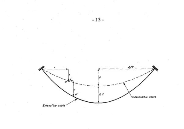
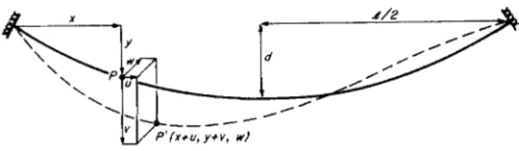
It ca.n be seen from Fig. 2 that an element at point P

in the inextensible profile, with coordinates (x, y), moves to a new

position at P' in the stretched profile, with coordinates (x

+

y

+

movements of the cable element respectively.

Provided that these movements are small, vertical

equilibrium of the eleme.nt in the stretched configuration is given by

d2

(H - ~H}-₂ (y+v)

=

dx

which can be integrated directly to give the parabola

1

wi~

Y

+

= (

T -

T

(1. 12)

(1. 13)

~H

where H* =

H.

parabola for the additio.nal deflection is found to be

H* wf3 {x (x)2}

v = ( 1 - H*) 2H

T -

T

Hence, the fractional increase in sag owing to cable stretch is

(1. 15)

.1/2

d

\Inextensible cable

Figure 2 Definition diagram for elastic parabola.

y

2

I

2

Y =..1_/2H -H ₂₄ (<

*

In order to evaluate H.,,, _.,.. recourse must be made to the cable equation which relates the stretching of the cable element

to the geometric displacements which it undergoes. In the present

context the equation reads

(H - .6H) ( ddxs

)s

=

+

+

.!..

EcAc dx dx dx 2 (1. 16)

where Ee is Young's modulus and Ac is the area of the cable. This

equation is of fundamental importance and is accurate to the second

order of small quantities. A derivation of the general cable equation

can be found in Appe.ndix II.

The displacements u and v are zero at each end of

the cable,

*

~:

integra-tion by parts of Eq. 1. 16 yields

(1. 17)

where Le is a virtual length of the cable defined by

After substitution, integratio.n and rearrangement the

following cubic is obtained from Eq. 1. 17

where

The dimensionless variable, A2 , is the fundame.ntal

parameter of the extensible cable. It takes account of the effects of

initial cable geometry and cable elasticity and will arise repeatedly

throughout this thesis.

Equation 1. 18 can be solved in standard ways, but a

graphical solution is convenient here. Figure 3 shows that H.,, must

_...

lie between

0 < H _~~

<

an intuitively obvious result. Consider now the two limits for

>..2 :

(i) :>._2 large (i.e. :>._2

>

This covers most freely hanging cables which have

small, although appreciable, sag to span ratios. To sufficient

accuracy Eq. 1. 18 then becomes

from which

I

!::::..(

₊

~)

( 1. 19) 1

The corresponding result from Rankine's approximate theory (as

reported by Pugsley(l O)), may be rearranged to

d,,,

_...

which is somewhat larger.

1

Consider the following example which could apply to

a free-hanging cable of a long- span suspension bridge.

Example 1

Cable properties: 1 = 915 m (3000 ft); w = 4. 4 kN/m

(300 lb/ft); Ee= 180 X 106 kN/m2 (26 X 106 _{psi); Ac= O. 161 m2}

(250 in2 ); sag ratio (initial geometry)

=

Hence

and consequently

from which

A. 2

=

03

>>

o o

1 H* ~ 170

D.d ~ 0. 455 m (1. 49 ft)

In a more realistic exarp.ple attention would have to be paid to the

possible influe.nce of the towers and side-spans.

(ii)

A

A

<<

Cables for which

A

case

~

Ee is small). Some care has to be exercised in taking the limits of

Eqs. 1. 13 (or 1. 14) and 1. 18 as A.a approaches zero. In such cases

(I. 20)

1

{d~M)

=if

{(~)(E~J(~ef

Three separate situations may be isolated, in each of

which

A.

~)

taut, flat steel cable, it is seen that C.d-+ 0, as expected. If, for

some cable, both

(~)

Alt ernative y, . 1 i"f

(wH:£)

impor-tance. Indeed, the third case can be correct only in a qualitative

sense since the assumption of small additional deflections, on which

the analysis is based, is clearly violated.

It is noticed from Eq. 1. 20 that a substantial change in

tension occurs when A.a is very small. This could be important in a

practical situation involving taut, flat steel cables if a procedure was

However, this procedure is usually impracticable since the unstressed

length of such a cable is only a minute fraction longer than the span

and problems of accurate measurem:e nt and construction would

cer-tainly arise. Normally, the construction of such a cable would be

effected by placing it in jacks, prestressing the cable to a given

pre-tension, and then anchoring it off. Since the weight and span of the

cable are known, the sag in the free -hanging position is found directly

from the inextensible theory, Eq. 1. 6.

It may be concluded that the theory of the elastic parabola

will find an application primarily in the construction of the cables of

suspension bridges and possibly in the construction of large, overhead

electric power lines. The approximate results given by Eq. 1. 19 may

be used with confidence for such problems. In most other practical

situations, the stretching of the cable in its free-hanging position may

2. Parabolic Cable Under Applied Loads

After the discovery of the catenary, the first work which

considered the behavior of a free-hanging cable under the action of an

applied load was that of James Bernoulli(lS) at the end of the

seven-teenth century. Using geometrical principles, as was common at

that time, he investigated the response of a catenary to a central

force.

It was not until 1796 that Fuss(lS) derived the general

equations of equilibrium, in Cartesian coordinates, for a cable

element under any type of force.

Later, around the middle of the nineteenth century, several

papers appeared in connection with the design of suspension bridges in

which analyses were presented for the behavior of a heavy, parabolic

cable under various types of applied loading. These theories were

developed partly by Rankine in 1858(lO), but mainly by an anonymous

writer in 1860 and 1862(lO). It was realized at this time that the

response of the cable was non-linear. Successive equal increments of

load were seen to cause successive increments in the corresponding

deflection, each smaller than the last. This non-linear stiffening

effect was later discussed in some detail by Pugsley(l O). These later

theories have been presented in book form by Pugsley(lO).

More recently, with the advent of the digital computer,

numerical solutions have been presented. For example, 01_{Brien( 9 )}

has shown how numerical techniques may be employed to obtain

gen-eral solutions to suspended cable problems. Buchanan(!) has

perturbation methods. The digital computer is sometimes an

essential tool in analyzing complicated problems, however, its use

is not required to solve the problem at hand.

In the analyses to be presented here, the equations of

equilib-rium are solved in a straightforward and physically meaningful

man-ner. Compatibility of displacements will be satisfied by a cable

equation which, in general, will allow for terms up to and including

the second order of small quantities. Thus, general results are

derived which are accurate to the second order of small quantities.

Simplifications are then made to the general theory; tbe solutions are

linearized and they are also adapted to apply to cables which are

initially taut and flat.

a. Point load on cable

To begin with, it is assumed that the shape of the cable,

in its free-hanging position, is given by the parabola

where any initial effects, owing to cable elasticity, have been

ac-counted for.

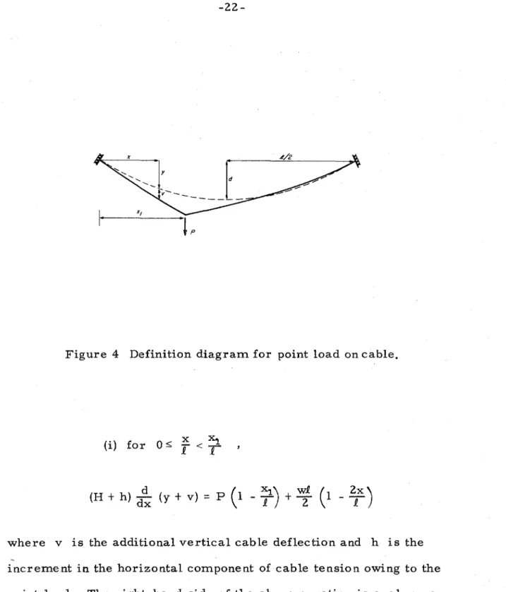
Consider a point load P acting at a distance x₁ from

the left-hand support (see Fig. 4). Provided that the additional

move-ments of the cable are small, so that the slope of the cable remains

small, vertical equilibrium at a cross section of the cable requires

Figure 4 Definition diagram for point load on cable.

X X1

(i) for o~

T

<r

(H

+

+ )

(1 -

~1)

+

(1 -

dx Y v .x. .x.

where v is the additional vertical cable deflection and h is the

increment in the horizontal component of cable tension owing to the

point load. The right-hand side of the above equation is analogous

to the shear force in a simply supported beam of uniform weight under

(H

+

=

(1 -

~

dx J. dx

Similarly it is found that

( .. ) f X1 < X

<

11 or

T

T

(H

+

=

~

(1. 21)

( 1. 22)

Equations 1. 21 and 1. 22 are then integrated and, after

the boundary conditions have been satisfied, the dimensionless

equations for the additional vertical cable deflection are found to be:

where

(i) for 0 < _{- J _ - J . '} ~ < ~

Xl X

(ii) for

T

T

<

v

v*=(i:)

= -

*

p

p =

-*

( 1. 23)

The non- linear nature of the response of the cable to the applied

In order to complete the solution, h.,. must now be _,,.. evaluated. Use is made of the cable equation, where terms up to

and including the second order of small quantities have been retained

(see Appendix II).

J

.P..

1.P..

[.P..

_

iY.

- du

+

+

Z

(

0 0 0

Since

*

w 1 dv 2

1

.P..

J.P..

= H v dx

+

z (

0 0

Under point loading

(~:)

position of load application and the last integral above, when

inte-grated by parts, gives

_!.{dv v 2 dx

This result may now be substituted into Eq. 1. 25. After Eqs. 1. 23

l

and 1. 24 have been substituted into Eq. 1. 25 and the integration has

This equation may be rearranged to the standard form for a cubic

h!

+

(2

+

~:)h~~

+

(1

+

~

2

(

(~

1

)- (~

1

)2)

+

=

o

( 1. 26)

This cubic is of the form

z3

+

+

=

where a, b, c are positive, real quantities. Accordingly, from

Descartes' ''rule of signs", there is just one, positive real root of

Eq. 1. 26. This root is the required value of h*.

The cubic can be solved exactly using the requisite

forms of Cardan' s equations (see, for example, U spensky<20

».

For a given problem it is clear that h ... depends not "I'

only on P * and

f,

for cable geometry and elasticity. Also, it may easily be shown

that, for given values of P * and >.,2 , h* is a maximum when

Xi=~

.

The variables P J , and A.

2

may take on any value, large or small,

...

provided that the slope of the cable remains small.

A knowledge of the small, longitudinal cable

move-ment induced by the loading, may be important in some applicatio.o.s.

These movements may be calculated from the cable equation and in

where

and

(1. ) f _or Q ...,.

_{""T - T'}

Lx

h*L

e

Xi X (ii) for

T

T

is the value of v,,, at ,,, x1 ,

(1 -

~)}

v*

d

(xJ

f_ I

(Xi)} V* _{f. J 2}

P,:, V>:i: I

+

-2-Lx

+

(f) { (;) -

+

j (:)}

J

The above results are general and will provide

(1. 27)

(1. 28)

accurate solutions for practical problems in which the effects of a

point load on a parabolic cable have to be assessed.

Two useful simplifications are possible for the general

theory. ln the first the solutions are linearized, in the second the

solutions are simplified to provide results for cables which are

(1) Linearized theory

The problem is linearized by neglecting all

second order terms which appear in the differential equations of

equilibrium and in the cable equation. This requires that the term

dv 1 [.R.(dv\2

h dx be left out of Eqs. 1. 21 and 1. 22. The term

z

dx / dx

must also be removed from Eq. 1. 25. As a consequence, the

equations for v* read:

(1.) f _or Q _s;

T

T '

(1. 29)

X1 X

(ii) for

T

T

s

(1.30)

The cable equation is reduced to

hLe

l.R.

- - =

0

(1.31)

and after substitution, integration and rearrangement the following

linearized expression is obtained for h*

Usually these linearized solutions will be

accu-rate only as long as P .... remains small. In fact, when A 2 is large

'•'

P,,, should not be greater than about 10-1 if the equations are to be

'•'

accurate to within 10%. However, when :x_2 is small, larger values of P* are admissible. In practice, steel cables are invariably used

for structural purposes. Thus, changes in )._2 _{are brought about}

mainly by changes in the cable geometry. Small values of

A

correspond to very flat-sag cables, while large values of :x_2 ,

reflecting the relatively inextensible nature of the steel material,

correspond to more appreciable sag ratios ( S 1 :8).

For taut, flat cables :x_2 << 1, and it can be seen from Eq. 1. 32 that h.,, ....

o.

"' Hence Eq s. 1. 29 and 1. 30 reduce to

those of the classical linear theory of the taut string.

For cables, such as those of the suspension

bridge, where the sag ratio is of the order of 1: 10, A 2 >> 1 and

This result is reported by Pugsley(lO).

O.ne final point, which is of interest for the

linear cable, concerns the overall maximum additional deflectio.n

under a point load. For a given value of

f

deflection occurs at x_{1 •} Since

T

and 1 , the overall maximum depends on position. To locate this

in either Eq. 1. 29 or Eq. 1. 30 to give

v,,, _,,. = (1.33)

Setting the derivative, with respect to

~

zero indicates that possible turning points exist at

(i) Xl - 1

y-z:

(ii)

i "

~

{I

(I -

~

(I

+

~;

) )

!; }

For real roots (which are equally spaced about mid-span), it is

necessary that

A.a

This is an important criterion and leads to the following observations:

(i) If A. a ~ 24 ,

then v..,,, has an overall maximum when _....

(1. 34)

When

A.2 >>

11 )

~l

~

(1=f)3)=o.211, o. 789

This latter result is reported by Pugsley (l 0

>.

1 ( 12)

v*

=IT

+A.a

and when

xa

>>

(ii) If

xa

*

( 1. 36)

and this overall maximum value of v * is

(1. 37)

When

A.a

Therefore, for the linear parabolic cable, the

overall maximum value of v*, owing to a point load, occurs at the

point of loading and lies between

It may be concluded for the linear cable that

both the overall maximum value of v

*'

Xl

T ,

.x_2 •

non-linear problem since the solutions will depend on F_,, _.,. as well as

The linearized solutions presented here will be

accurate provided that P.,, ,...., 10-1 • If P,.... is larger, as it will often

"l... "l"

be, then second order effects must usually be considered. There is

some difference of opinion on what second order terms must be

retained. In the general theory of this thesis, all second order terms

are retained. However, Pugs ley(l O) allows for second order terms in

the equations for cable deflection, but both second order effects and

the effects of cable elasticity are removed from the cable equation.

While this appears a reasonable assumption for such problems as the

response of a suspension bridge cable to a point load (see Example 2),

it is somewhat inconsistent and will lead to inaccuracies in other

situations (see Example 3). Incidentally, if the cable is assumed

inextensible from the outset (as Pugsley has done), there is no way

that the linear theory can give the correct result as the initial cable

(2) Taut, flat cable

Since in this situation the cable is initially flat

(or, in reality, nearly so), y

=

vertical cable deflection are:

X Xl

(i) for

o

<

T

T

v..,,,

=

1 { (1 -

~1)

: }

"I' ( 1

+

(ii) for Xl < ~ < 1 f. - J.

-The cable equation becomes

11.R.

=

2

(dx) dx

0

(1. 38)

(1. 39)

( 1. 40)

.

d

Since dx₂ = 0, the cable equation may be reduced, after integration by parts, to

(1. 41)

and differentiation and substitution of Eqs. 1. 38 and 1. 39 in Eq. 1. 41

and rearrangement gives

In this situation A2 is always very small since (

7i

r

_.•.

A2 P*2 is not necessarily small. If P~:c is small, then h* -> 0, and

the classical results for the linear taut string are obtained.

Equation 1. 42 has an exact solution of the form

1 { 1 }

2

h*

=VA

~

-

3

where

A=-q+j9-:.+£

and

_ X

2

{

(x

1

~

_ (x1)2

}P!

2

'-1

As expected, it can be shown that

_{;{A> 3,}

_;(A

=

₃

X1

P.,, = 0, or 71 = 0, 1.

'f" ..t'..

The results given by Eqs. 1. 38, 1. 39 and 1. 42

may be rearranged to give a standard, classical form. If the value

of v at x

=

O·,

(1. 44)

(1. 45)

1 . (3)

When x₁ =

2 ,

These two latter solutions are particularly useful

if

o ,

previous formulation is of most use. The classical formulation, as

given by Inglis, is obtained by considering equilibrium at the position

of load application and then applying a binomial series expansion to

Pythagoras' theorem in order to estimate the relationship between

the deflection and the stretching which the inclined cable components

undergo. This method of solution is straightforward only when a point

load is applied to a flat cable. By comparison, the other approach

outlined here is a particular adaptation of the general theory which

can be used readily in other situations where the classical formulation

would be extremely difficult to apply.

b. Examples

As a means of illustrating the theories derived so far,

consider the following examples.

Example 2

The first segment of the deck of a long-span suspension

bridge is to be lifted into place at mid-span (for example, see the

photograph on p. 19). It is required to find the additional deflectio.n

at mid-span and the increment in the horizontal component of cable

free-hanging position.

1. = 915 m (3000 ft); w = 4. 4 kN/m (300 lb/ft); Ee= 180 X 106

kN/m2 (26 X 106 _{psi); Ac= O. 161 m2 (250 in2 ); sag ratio (in}

free-hanging position)= 1:12

The weight of the segment, per cable, is

P = 890 kN (200, 000 lbs)

Hence, ).2 = 2 X 103 , { = O. 5,

becomes (Eq. 1. 26)

P,.,

_....

=

h~ ...,,...

+

+

and the solution is found to be

h* =

o.

This may be compared with the linear theory (Eq. 1. 32) which gives

h.,,

_....

=

o.

Although this is little different from the more exact theory, the close

agreement is misleading. For this problem the relationship between

additional cable tension and applied loads appears essentially linear,

but the relationship between additional deflection and applied load is

not linear.

from which

The additional deflection at mid-span is, (Eq. 1. 23)

v

=

o.

*

In a more realistic example the possible influence of the towers and

sidespans would have to be assessed.

Example 3

A 11_{flying fox" is used to transport materials across a}

ravine. In its free-hanging position the cable spans 91. 5 m (300 ft)

with a ratio of sag to span of 1 :50. It is required to find the additional

horizontal component of cable tension and the additional cable

deflec-tion when a point load of 17. 8 kN (4000 lbs) is carried at mid-span.

Properties of the cable are: w

=

=

104 Xl06 kN/m2(15X106 psi); Ac= 5. 06 X l0-4 m2 (0. 785 in2 ).

Hence, A 2

=

T

o.

_,,.

=

From the general theory (Eq. 1. 26) the cubic for h, ... _,,,

becomes

h~. "f"

+

+

=

and the solution is

h, ... = 4. 65

"''

If the theory of the taut, flat cable is applied, the cubic

for h* becomes (Eq. 1. 42)

h_...(l _,,.

+

h_...

=

"\'

On the other hand, the linear theory (Eq. 1. 32) gives

In this problem the general theory is indispensible if the correct

solu-tion is to be obtained.

The additional cable deflection at mid-span is

(Eq. 1. 23)

v.,,= 0.0237

'I'

from which

v

=

Under this loading the sag of the cable has almost doubled but, since

the cable slope is still small, the result is re liable.

(c) Experiments on a taut cable

In order to check the accuracy of the theories presented

for the response of a cable to a point load, it was decided to carry out

a short experimental program. A flat, taut cable was chosen since it

is the easiest to experiment on. Also, it was felt that, since the

theory for the taut cable is closely related to the general theory, good

agreement here between the theory and experiment could reasonably

be construed as verification for the general theory.

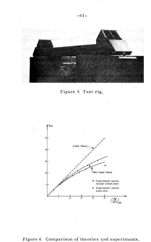
Consequently, a small rigid test rig was constructed

which had a clear span of 91. 5 cni (3 ft). See Fig. 5. The cable

was anchored at one end and passed over two rigid uprights before

being anchored in a nut and bolt device at the other end. The initial

cable tension was adjusted by this device.

Two types of cables were tested. One consisted of

In each case the experimental procedure employed was

as follows. The cable was placed in the rig and pretensioned to some

value H. This initial pretension was calculated by measuring the

deflection caused by hanging a small weight from the mid-span point.

The linear theory was then applied to determine H. Successively

larger weights were then hung from the mid-span point and the

corresponding deflections were measured.

The equation governing load and deflection at mid-span

is (see Eq. 1. 38)

1 Pl

v

=

(1

+

'•'

where h,,,. is determined from Eq. 1. 43. When P is small, h,,,~ 0,

•

and the initial pretension can be found from

H =Pf.

4v

The results have been tabulated and also presented in

graphical form to facilitate comparison with the linear theory and the

second order, non-linear theory.

(i) Multistrand cable

The cable used was a Bethlehem steel aircraft cord

of diameter O. 12 cm (3

I

=

kN /ma (15 X 106 psi); w = 0. 0553 N /m (O. 0038 lb/ft). Because the

cable comprised numerous twisted strands it did not kink at the

uprights and was able to move freely over them. Consequently, the

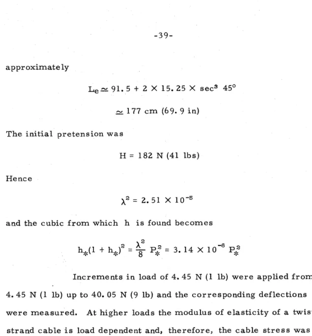
approximately

Le~ 91. 5

+

~ 177 cm (69. 9 in)

The initial pretension was

H

=

Hence

A.

₌

and the cubic from which h is found becomes

2 A ,2 2 -6 2

h*( 1

+

8

x

Increments in load of 4. 45 N (1 lb) were applied from

4. 45 N (1 lb) up to 40. 05 N (9 lb) and the corresponding deflections

were measured. At higher loads the modulus of elasticity of a twisted

strand cable is load dependent and, therefore, the cable stress was

kept well below the elastic limit to avoid any unnecessary

complica-tions.

Table 1 lists the experimental results and the results

from the linear and non-linear theories. Figure 6 shows dimensional

plots of the experimental results and the theories.

It is clear that there exists excellent agreement between

the experimental results and the non-linear theory. Agreement

between the linear theory and the experimental results is poor at all

but the smallest loads. The linear theory does not allow for additional

Table 1

Comparison of theory and experiment for the twisted strand cable

Experiment Non-linear theory Linear theory

p _{v H+h} v H+h v H

(N) (cm) _{- 4v} Pi (cm) (N) (cm) (N)

(N)

0 0 182 0 182 0 182

4.45

o.

o.

8. 90 1. 03 197 1. 03 197 1. 12 182

13.35 1. 43 214 1. 44 212 1. 68 182

1 7. 80 1. 78 229 1. 79 227 2.24 182

22.25 2.06 247 2.07 244 2.80 182

26.70 2.34 261 2. 35 260 3.36 182

40.05 2.65 345 2.97 308 5.04 182

Table 2

Comparison of theory and experiment for the piano wire

Experiment Non-linear theory Linear theory

p _{v H+h v H+h v H}

(N) (cm) _{- 4v} Pl (cm) (N) (cm) (N)

(N)

0 0 l.16 0 116 0 116

4.45

o.

o.

o.

8.90 1. 59 127 1. 61 126 1. 76 116

13. 35 2. 19 140 2. 19 139 2.64 116

17.80 2. 66 153 2.70 152 3.52 116

Vcm

5

4

3

2

Figure 5 Test rig.

. h /

Lmear t eory----... /

y

/

/ /

/ / /

/ / / .~

/

_ /

_...---/ _...---/ ./~

..

/ /

....-•

/~,./ Non-linear theory

/ ,,-::."

/+/./

/9v

.J'ii

/

• Experimental results,

twisted strand cable

• Experimental results,

• piano wire

2 3 4 5

will be noticed that the non-linear theory overestimates the actual

deflection for the 40. 05 N (9 lb) load. It is concluded that at this

load, the helical strands of the cable are starting to straighten out,

with a consequent rise in the modulus of elasticity of the cable.

(ii) Piano wire

The cable used here was a single strand of Malin' s

Musical Wire ( # 5) of diameter O. 0355 cm (0.012 in) and properties:

Ee= 207 X 106 kN/m2 (30 X 106 psi); w = 7. 63 X 10-3 N/m

(5. 22 X 10-4 lb/ft). It was noticed that this piano wire formed kinks where it passed over each upright. Under load there was no cable

movement past the uprights and consequently the virtual cable length

Le was taken to be just the clear span

Le = 91. 5 cm (3 ft)

The initial pretension was 116 N (26. 2 lbs). Hence

x

_6.

and the cubic from which h is found becomes

Increments in load of 4. 45 N (1 lb) were applied from

4. 45 N up to 22. 25 N (5 lb), and the corresponding deflections were

measured. The cable stress was always well below the elastic limit.

Table 2 lists the experimental results and the results

from the linear and non-linear theories. Figure 6 shows dimeqsional

As in the previous experiment, there exists excellent

agreement between the experimental results and the non-linear theory.

Again, the linear theory, which does not allow for additional cable

tension, predicts deflections which are too high.

Conclusions

Excellent agreement was obtained between the

non-linear theory and the experimental results. The experimental results

confirm the theory as applied

to

general theory.

d. Uniformly distributed load on part of cable

Consider a uniformly distributed load of intensity p

per unit length applied along the span froin x = x₂ to x = Xs. (see Fig. 7.)

+

+

+

+ + + +

+ +

+

I

By again exploiting the analogy which exists with the

simply supported beam, vertical equilibrium at a cross section

requires that:

x 43 (i) for

o ::;;

T ::;; T ,

(H

+

~:"

(1'- -1"-) -

~

(G•)

2

-

('f )

) } - h

~

(ii) for

]a

~T ~

7 ,

(H

+

~:"

G' _

n-

~

(

(i)" _

(??)") }-

~

Xs x

(iii) for -_,f ~ -_P. ~ 1 ,

(H

+

~: ~

~

(~)

2

-

('?)

) } - h

~

( 1. 46)

(1.47)

( 1. 48)

After integration and adjustment for the requisite boundary conditions,

the following dimensionless equations are obtained for the additional

vertical cable deflection:

(i) for 0

:s: :

s:

? ,

v*"

i,,,l [ {

G· -

'?)-

~

(G")"

-(?)")

}C;')- ::

0

G')-W)°)]

(l.49)

1

[ { - .!_

(Xa\2

+

(Xs)

(x) _

(x)2 _

.!.((x

3

_~

_

(~}

) (x~}

2 J_) \J. £ 2 J_ 2 J_ I J_ ,' J.;

v

*

+

J

h* ( 1

(x~

(x)

2

)

J

- P,:,

2

T, -

2

T

(iii) for

7

~

;

v*

=

h,.l

[HG•)-(]"-)"} (

::(~

(;)-1 (:)")]

where v_...

_.,

=

""

- p P~, - w •

The increment in the horizontal component of cable

tension, h, is found from the cable equation (see Appendix II) which,

since both

~i

~:

(1. 52)

After substitution of Eqs. 1. 49, 1. 50, 1. 51 into Eq. 1. 52, integration

and rearrangement, the following dimensionless cubic for h.., is

-··

obtained

-A; {

~

( (":)" -

G•)") -

~

(

(":)° -

(??-)")}

-A;

{HG•)"+

(?)') -

(7)

(]a)" -

~

(

(i)" -

(?-)") "}

_pjl

This general cubic is of the form

z3

+

₊

where a, b, c are positive real quantities. From Descartes' "rule

of signs11 _{there is just one, positive root to the above equation. This}

root is the required value of h*.

As before, the general solution for h,0; can be obtained ,,. using the requisite form of Cardan's equations.

It will be noted that there is a symmetry in the

co-efficient of the cubic involving ~ and Xs • As is to be expected,

the solution of the cubic is the same if x3

=

=

X:;

=

=

If the loaded length (X:; - ~) is allowed to become

very small, whiie p(:xs - Xa) remains finite, it is easily shown that

Eq. 1. 53 reduces to Eq. 1. 26, the result previously obtained for a

point load on the cable.

It can also be shown that whe.n p,0; and

A.2

"'

h.,_ is a maximum when the loading is placed symmetrically about

"'

mid-span.

Equations from which the longitudinal cable movements

can be found will not be given here. These small movements can

be calculated from the cable equation by employing the same procedure

as was used to obtain Eqs. 1. 27, 1. 28.

The above solutions are accurate to the second order

of small quantities. They will find particular application in the

deck is being hung in position. Here, use of the general non-linear

theory is essential since the deck load is usually many times greater

than the weight of the cables and >._2 is large. At this stage the stiff-ness of the deck is negligible since, in order

to

between adjacent segments of the deck until near the end of the

con-struction of the deck.

In certain situations the theory can be simplified and

these are now briefly considered.

(1) Linearized theory

In keeping with the approach given in the section on the point load on a cable, all second order terms are dropped from

the cable ~quation and the deflection equations. Consequently, the

equations for additional, vertical cable deflection are:

(i) for

o

~

;.

~

]a-v*

= [

{G· -

i')-

~

(

G•)" -

(':')")}(¥)- :: (

~

(T)-

~

G')")]

( ) f _{ii or} ~ _{i. ::..} ...

_T

_s:

_T

Xs

v,

~

('?)

+

('?)

G')-

Hn" _

~

(

('?) _ (i')")

~x)}

-:: (

~

(:) -

~

G'J)

J

(iii} for Xs _.R. ~

_T

_,

(1. 54)

(1. 56)

The cable equation is reduced to

(1.57)

and after substitution, integration and rearrangement the following

linearized, dimensionless expression is obtained for h.,,

'•'

h.,, _,,, =

(1. 58)

Because of the linearity of the problem, this result could also have

been obtained by integrating Eq. 1. 32 directly.

These solutions will be accurate for all A,2

provided p* is small, near 10-1 •

Again, if A,2 _{<< 1, as in taut, flat cables, h.,, ... 0}

""

and the classical results of the linear, taut string are obtained.

For cables, such as those of the suspension

bridge, where the ratio of sag to span is of order 1:10,

A.

_>>

1 and

which is the ·result obtained if the cable is assumed inextensible, and

(2) Taut, flat cable

A considerable simplification results here since

y

=

(i) for 0 s: ; s:

-?--"2 .... x ~

(ii) for i. .;::,

T

(1. 59)

v~:

=

J

h,~)

-i

(~)2

+

(~

3

)

(T)-

~

(;)2 _

~ ((~

3

)2 -(~)2)(;)]

(iii) for Xs

s:

i. i.

The cable equation may here be reduced to

and substitution, integratio.n and rearrangement gives

h* ( l

+

hs

=

~

{

~

(

(7J

+

c;) (";)'

-

~

( G")" G")"

)"}p*

(1. 60)

(1.61)

(1. 62)

where here

This is a cubic of the same form as Eq. 1. 42. The parameter )._a

is always very small since (

7f

)a

However, p* is usually large so that the product p*

A.

necessarily small. If p* is small then h* .... 0, and the classic al

re suits for the linear, taut string are obtained.

This cubic has an exact solution of the form

(1. 64)

where

and

r

= - ; '

s

= -

i1 -

~a

{

t (

(~

2

J

+

(~J)

-({)

(7)a

It can also be shown that

~

~

or

f

=

1

:;;B

3

This theory will find an application in the

analysis and design of cable roof structures which are rectangular

in plan. If one side is much larger than the other side then it is

cables are initially taut and flat (as wi 11 often be the case), it is a

simple matter to calculate the additional deflections and tensions

developed after the (usually} light and flexible roof is hung from, or

made continuous with, the cable system.

e. Examples

Consider the following examples which illustrate the

results obtained for the respo.nse of cables to distributed loads.

Example 4

It is required to calculate the additional tensions and

deflections induced in the cables of the long-span suspension bridge

of Example 2 (p. 34) as construction of the deck proceeds. In

particular, the additional horizontal component of cable tension and

the additional vertical cable deflection at mid-span are to be evaluated

for:

(i) deck in place over the central half of the span,

(ii) deck in place over all the span.

The distributed weight of the deck is

p = 5. 84 X la4 N/m (4000 lb/ft), per cable

and it is assumed that during construction the deck has no flexural

stiffness. Other properties are as given in Example 2.

(i) deck in place over central half of the span

Here

\ 2 = 2

x

II.

r= .

.

X3

T

=

o.

'l'

h!

+

+

"l' ...,,... ""'

from which

The additional deflection at mid-span is (Eq. 1. 50)

v*

=

=

If the cables were assumed inextensible, and the second

order term was left out of the cable equation, then h* would have a

value given by (see p. 48)

h.,,. _,,.

=

which is quite close to the value given by the general theory.

However, the cables are not inextensible. I.n fact,

under this loading, the cable length has increased by an amount

which is far from negligible. The 11_inextensible11 _{theory gives a good}

result because two terms in the cable equatio.n, namely

111

and 2 (d:) dx

0

are approximately equal in this case. Consequently, the value of h*

found from the equation

1

-is close to the value given by the general theory.

(ii) deck in place over all the span

Here

;x,

₌

_x

xa

T

o ,

The cubic to be solved is

X3

r = l . O ' p,., .,, = 13.3

h:_

+

+

from which

h.,, _.,, = 12. 35

This may be compared with the result from the "inextensible" theory,

namely

h..., _{... ,....} = p...,

_..

The additic:;>nal deflection at mid-span is

from which

v =

o.

*

v = 5.43 m (17. 8 ft)

Therefore, in placing the deck on the mainspan, the cable sag has

increased from 76. 2 m (250 ft) to 81. 7 m (267. 8 ft). Each cable has

increased in length (from its length in the free-hanging position) an

amount

~L ~ 2.42 m (7. 95 ft)

The fractional increase in cable length is

~L - O. 0026

-y:;--which is much smaller than the fractio.nal increase in sag of

b.d

d

=

o.

Example 5

A factory, the roof of which has plan dimensions

of 91. 5 m

x

by, and made continuous with, a parallel network of cables which

span the shorter side at a spacing of 6. I m (20 ft). The cables

are anchored into rigid supporting frames as shown in Fig. 8.

/ Cob/es and roof

Figure 8

As a part of the preliminary design of the roof

structure, consider the following possible structural solution:

Steel cables, 3. 8 cm (1. 5 in) in diameter, are