Discharge hydrograph estimation at upstream ungauged sections by coupling a Bayesian methodology and a 2 D GPU shallow water model

Hydrol. Earth Syst. Sci., 22, 5299–5316, 2018 https://doi.org/10.5194/hess-22-5299-2018 © Author(s) 2018. This work is distributed under the Creative Commons Attribution 4.0 License.

Discharge hydrograph estimation at upstream-ungauged sections by

coupling a Bayesian methodology and a 2-D GPU

shallow water model

Alessia Ferrari1, Marco D’Oria1, Renato Vacondio1, Alessandro Dal Palù2, Paolo Mignosa1, and Maria Giovanna Tanda1

1_{Department of Engineering and Architecture, University of Parma, Parma, Italy}

2_{Department of Mathematical, Physical and Computer Sciences, University of Parma, Parma, Italy} Correspondence:Alessia Ferrari ([email protected])

Received: 8 March 2018 – Discussion started: 27 April 2018

Revised: 2 August 2018 – Accepted: 20 September 2018 – Published: 16 October 2018

Abstract.This paper presents a novel methodology for esti-mating the unknown discharge hydrograph at the entrance of a river reach when no information is available. The methodology couples an optimization procedure based on the Bayesian geostatistical approach (BGA) with a forward self-developed 2-D hydraulic model. In order to accurately describe the flow propagation in real rivers characterized by large floodable areas, the forward model solves the 2-D shal-low water equations (SWEs) by means of a finite volume ex-plicit shock-capturing algorithm. The two-dimensional SWE code exploits the computational power of graphics process-ing units (GPUs), achievprocess-ing a ratio of physical to computa-tional time of up to 1000. With the aim of enhancing the com-putational efficiency of the inverse estimation, the Bayesian technique is parallelized, developing a procedure based on the Secure Shell (SSH) protocol that allows one to take ad-vantage of remote high-performance computing clusters (in-cluding those available on the Cloud) equipped with GPUs. The capability of the methodology is assessed by estimat-ing irregular and synthetic inflow hydrographs in real river reaches, also taking into account the presence of downstream corrupted observations. Finally, the procedure is applied to reconstruct a real flood wave in a river reach located in north-ern Italy.

1 Introduction

reverse form of the Saint Venant equations (e.g. Eli et al., 1974; Szymkiewicz, 1993; Dooge and Bruen, 2005; Bruen and Dooge, 2007) and the back-oriented application of hy-drological routing schemes (e.g. Das, 2009; Koussis et al., 2012; Koussis and Mazi, 2016). Beyond the approximations introduced by the hydrological routing schemes, the afore-mentioned procedures were applied to simplified reach ge-ometries and flow conditions. In almost all cases, especially considering downstream information affected by errors, in-stabilities and spurious oscillations appeared; low-pass filters with subjective parameters were sometimes used to dampen the estimated inflow fluctuations. D’Oria and Tanda (2012) and Zucco et al. (2015) provide additional references and de-tails on the reverse flow routing problem.

In addition to the above procedures, the estimation of an unknown upstream flow hydrograph based only on down-stream information (observations) can be performed via op-timization methods. These techniques aim at finding the upstream flow hydrograph that, routed downstream, best matches the available observations. D’Oria and Tanda (2012) solved the reverse flow routing problem by adopting a novel Bayesian geostatistical approach (BGA) as an optimization procedure that considers the flow hydrograph as a continuous random function that presents autocorrelation. The authors showed the capability of the BGA methodology, in combi-nation with a forward hydraulic model, to estimate the dis-charges in an upstream-ungauged section based only on an available downstream flow hydrograph: the solution was sta-ble also in the presence of corrupted downstream flow values. The forward model, which solves the 1-D Saint Venant equa-tions, was considered already implemented and calibrated and was able to describe the hydraulic routing process with sufficient accuracy. The BGA method was further extended in order to adopt stage hydrographs instead of discharge ones as downstream observations (D’Oria et al., 2014). Saghafian et al. (2015) identified the upstream hydrograph of a river reach given the downstream one by using a genetic algorithm coupled with a forward hydraulic model that solves the 1-D Saint-Venant equations under the kinematic wave approxi-mations. Only some minor oscillations and instabilities oc-curred during the inversion, but the authors applied the pro-cedure to a rectangular prismatic channel, and no errors were added to the downstream observations. Zucco et al. (2015) investigated the reverse flow routing process in natural chan-nels and estimated the discharge hydrograph in ungauged sections by means of a genetic algorithm coupled with a sim-plified routing model. The parametric forward model was based on the continuity equation written in a characteristic form, lumped over the entire river reach, and on simplified rating curves at the channel ends. In addition, the unknown inflow hydrograph was assumed to be distributed in time as a Pearson type III function with three parameters, thus pre-venting the possibility of estimating real flood waves with irregular shapes (e.g. multi-peak hydrographs).

All the previously cited works adopted 1-D hydraulic models or simplified hydrological routing schemes in combi-nation with different optimization procedures. Nevertheless, in many real cases, the complex hydrodynamic field gener-ated by the flood propagation cannot be accurately described under 1-D assumptions, and it is necessary to adopt schemes based on the 2-D shallow water equations, even if this poses the drawback of the computational burden and requires a de-tailed terrain survey. However, nowadays, bathymetric data can be easily obtained from high-resolution digital terrain models (DTM), and fast 2-D numerical models have been de-veloped. With the purpose of estimating the discharge hydro-graph in an upstream-ungauged river section, having water level information only in a downstream observation site, this paper extends the BGA methodology for reverse flow routing from D’Oria and Tanda (2012) and D’Oria et al. (2014) to a 2-D forward algorithm in order to model natural rivers with complex geometry, including flood plains and floodable ar-eas. With this aim, the stable, accurate and fast PARFLOOD graphics processing unit (GPU) code (Vacondio et al., 2014, 2016, 2017), which solves the conservative form of the 2-D shallow water equations on a finite volume scheme, is adopted as forward model and is coupled with the inverse estimation procedure. In order to reduce the computational time, the Jacobian matrix estimation procedure, which is the key point of the BGA method, has been parallelized. Addi-tionally, a host–server data management procedure has been implemented to exploit the computational power of remote large modern supercomputer and/or cloud HPC resources. The capability of the optimization procedure has been tested by estimating real or pseudo-real inflow hydrographs in nat-ural river reaches, where 1-D models cannot accurately de-scribe the flood propagation. Moreover, during the discharge estimation, the presence of downstream corrupted observa-tions has also been taken into account, since registered data at gauging stations are quite often affected by instrumental errors.

A. Ferrari et al.: Discharge hydrograph estimation at upstream-ungauged sections 5301 2 Theory of the Bayesian geostatistical approach

The optimization software adopted to solve the reverse flow routing problem is the bgaPEST (Fienen et al., 2013), which implements the Bayesian geostatistical approach of Kitanidis (1995), and it is developed according to the PEST (model in-dependent parameter estimation) software (Doherty, 2016). The bgaPEST is appropriate for solving inverse problems (in a context of a highly parameterized inversion), which are characterized by unknown parameters that are correlated to one another in space or time, for example, the discharge val-ues of a flow hydrograph. The first applications of the inverse methodology were related to the estimation of spatial param-eter fields in a groundwater context (Kitanidis and Vomvoris, 1983; Hoeksema and Kitanidis, 1984, among others), but later the method was adopted to evaluate unknown time func-tions in different areas (e.g. Snodgrass and Kitanidis, 1997; Michalak et al., 2004; Butera et al., 2013; D’Oria and Tanda, 2012; D’Oria et al., 2015; Leonhardt et al., 2014).

2.1 Bayes’ theorem

The crux of the adopted bgaPEST, as well as other methods based on the Bayesian approach, is Bayes’ theorem, which reads

p (s|y)∝L (y|s) p (s) , (1) wheresis the vector of the unknown parameters,yis the vec-tor of the measured data,p (s|y)is the posterior probability density function (pdf) ofsgiveny,L (y|s)is the likelihood function, andp(s)is the prior probability density function of s. Since the present work aims at estimating an upstream hy-drograph in an ungauged section, assuming the knowledge of downstream water levels, srepresents the discharge val-ues over time of the unknown inflow hydrograph, whereas y denotes the downstream water level observations. Follow-ing Eq. (1), the posterior pdf can be seen as a combination between a priori knowledge on the parameters (prior pdf), where a priori means that the observed data are still not con-sidered, and information about parameters contained in the measured data (likelihood function) (Glickman and Van Dyk, 2007). In the BGA method proposed by Kitanidis (1995), the prior pdf and the likelihood function are described by means of Gaussian distributions, and the best set of parameter sis obtained by maximizing the posterior pdf.

2.1.1 The likelihood function

The likelihood function L (y|s)in Eq. (1) characterizes the deviation between observed data and model results (Fienen et al., 2013). Starting from the results of the forward model, L (y|s)delineates how a particular set of parameterssis able to reproduce the observations y in space and/or time, thus accounting for the epistemic errors. The investigated inverse problem presents different sources of errors that are related

to the conceptual schematization of the inverse procedure, the numerical forward model, and the data measurement. In the likelihood function, the errors are assumed to be inde-pendent and identically distributed, with the zero mean and covariance matrix expressed as follows;

R=σ_R2I, (2)

whereσ_R2 denotes the variance that expresses the misfit be-tween observed and modelled data, andIis the identity ma-trix.

2.1.2 The prior probability density function

The prior knowledge about s (p(s) in Eq. 1) is limited to the definition of a mean value (unknown and estimated dur-ing the procedure) and a characteristic about the continuity and/or smoothness of the parameter field described through a covariance function. It furnishes a soft knowledge about the structure/shape of the unknowns and provides a regulariza-tion of the soluregulariza-tion; the prior pdf can also be used to enforce non-negativity to the parameters (D’Oria and Tanda, 2012). The prior mean is defined as:

E[s]=Xβ, (3)

whereEis the expected value,βis the vector of drift coef-ficients, andXis a known matrix of basis functions. In our case,βis a single unknown scalar, but different drift coeffi-cients can be used to introduce discontinuities in the stochas-tic function to be estimated (e.g. when the unknown parame-ters are likely to form distinct populations). For example, in the context of reverse flow routing problems, multiple values ofβ are adopted if more than one inflow hydrograph must be estimated at the same time (e.g. the inflow on both the up-stream branches of a river confluence). The matrix of the ba-sis function,X, links each unknown parameter with the cor-responding element ofβand, at the same time, specifies the model of the mean (e.g. constant mean, mean with a trend, etc.); in our case the mean is constant and thereforeXis a single vector of one (Fienen et al., 2008).

The prior covariance matrix of the unknown parameters Qssis then defined as

Qss=E h

(s−Xβ) (s−Xβ)T i

. (4)

In the context of geostatistics, the covariance matrixQssis a function of the separation distance (in time in this case) between the parameters and describes their deviations from the mean behaviour. Different functions can be adopted to describe the covariance. For example, it can be assumed as a linear function, represented through a limiting case of the ex-ponential covariance function (Fienen et al., 2008) according to the following relation;

Qss(θ )=θ lexp

−|d|

l

where d represents the vector of the separation times be-tween all the parameter pairs (di,j=ti−tj, withi,j =1,

. . ., Np, t denoting the time associated with each parame-ter andNpthe total number of unknowns),l a fixed integral scale (l=10maxd), and θ the slope (structural parameter) that governs the correlation between the discharge values of the unknown hydrograph. A different formulation (D’Oria et al., 2014) defines the prior covariance matrixQssby means of a Gaussian function characterized by two structural pa-rameters (σ_s2andl);

Qss(σs2, l)=σ 2 s exp  − d 2 l2 

, (6)

whereσ_s2 denotes the variance. The linear function (Eq. 5) enforces only continuity to the solution, whereas the Gaus-sian function (Eq. 6) also adds a degree of smoothness, but the final solution is still driven by the observations.

2.1.3 The posterior probability density function With the assumptions made, the likelihood and prior terms that compose the posterior pdf of Eq. (1) can be rewritten as follows (Fienen et al., 2009; D’Oria and Tanda, 2012; D’Oria et al., 2014);

L (y|s)=exp

−1

2(y−h(s))

T_R−1_(y−h(s))

, (7)

p(s)=exp

−1

2(s−Xβ)

T_Q−1

ss (s−Xβ))

. (8)

In the likelihood function, the term h(s) represents the modelled values in the same place and time as the available observationsy. Therefore, to evaluateh(s), a forward model of the considered river reach that is able to describe the hy-draulic routing process is required in order to provide the corresponding downstream water levels for a given set of pa-rameters.

Recalling that the aim of the inverse procedure is to obtain the vector of the unknown parameterss, as well as to quan-tify the uncertainty in the estimation, the solution is found by maximizing the posterior pdf or, more conveniently, min-imizing its negative logarithm (objective function) (Fienen et al., 2013).

In case a linear relationship between parameters and ob-servations (linear forward model) holds, a computationally efficient method to find the best estimatesˆof vectors(andβˆ ofβ) is obtained by introducing the vectorξ=(HQ_ssHT+

R)−1(y−HXβˆ)and solving the following linear system of equations (Fienen et al., 2009);

 



ˆ

s=Xβˆ+QssHTξ

HQ_ssHT+R HX XT_HT ₀

ξ ˆ β = y 0 , (9)

where H is the sensitivity (Jacobian) matrix, representing how the observationsyare influenced by each unknown pa-rametersi (D’Oria et al., 2015). However, for the particular

problem under investigation,h(s) is non-linear and matrix Htherefore depends ons. Following the quasi-linear geosta-tistical approach (Kitanidis, 1995), the relationship between observations and parameters can be successively linearized about a candidate solutionsk, wherekrepresents each

itera-tion;

h(s)≈h(s_k)+eHk(s−sk) . (10)

Then, a correction to the measurements is applied according to the following relation;

y_k=y−h(sk)+eHksk. (11)

Therefore, the sensitivity matrix is evaluated at each itera-tion as follows (D’Oria et al., 2014);

e Hk=

∂h(s) ∂s sk . (12)

Analogously to the linear system in Eq. (9), the linearized system is solved according to

e

HkQsseHT_k +R eHkX

XTeHT_k 0

ξ_k+1 ˆ β_k+1

= y_k 0 , (13)

and the next estimate of the parameters is evaluated by means of

esk+1=X

ˆ

A. Ferrari et al.: Discharge hydrograph estimation at upstream-ungauged sections 5303

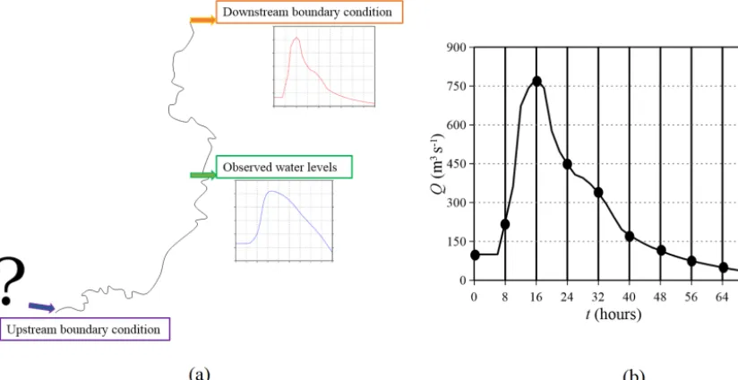
Figure 1.Definition of the reverse flood routing problem(a)and of the unknown parameters(b).

3 Description of the Bayesian estimation procedure

After having described the theory of the Bayesian geostatis-tical approach in Sect. 2, some operational information about the BGA inverse procedure is now illustrated. As mentioned in the introduction and illustrated in Fig. 1a, the goal of the adopted BGA methodology is the estimation of the discharge hydrograph in an upstream-ungauged river section (identified by a question mark in Fig. 1a), with information about water levels being observed in a downstream section (intermediate site in Fig. 1a). A boundary condition downstream of the ob-servation site must also be specified; this can be based on observed data or can be approximated extending the compu-tational domain far away from the intermediate section. The inverse method estimates theNpparameters (the vector of the unknown parameterssin Eq. 1) that originate from the dis-cretization of the upstream discharge hydrograph by means of time intervals, which are regular in this case (Fig. 1b).

The BGA algorithm solves the inverse problem by means of the following steps.

First, the unknown parameters and the structural ones are initialized. The first ones may all be assumed equal to a constant discharge value coherent with the considered river, whereas the starting values for the structural parameters are assigned so that the variability between contiguous parame-ters is small (flat solution, with a high degree of correlation); complexity is then introduced during the optimization pro-cess if supported by the data. The variance of the epistemic errors is assumed as being close to the expected one.

Assuming that the first guess for the unknown parameters is the upstream boundary condition, the hydraulic forward model is run, and the resulting water levels are extracted at the observation site. The simulation of a base run once a

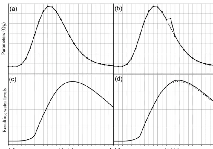
par-ticular set of parameters has been assumed (deriving from the initialization or from previous estimation steps) represents a mandatory step for the Jacobian matrix evaluation, which is performed at this point in the procedure in order to quantify how each observation is influenced by the variation of each estimable parameter. Particularly, Eq. (12) is approximated using a finite difference method; hence each element of the matrix is evaluated as the ratio between the variation of each observation (numerator) for given variation of each param-eter (denominator) with respect to the base run. Therefore, in addition to the base run, the hydraulic forward model is further run as many times as the number of parameters to estimateNp. With each run, a single value of the upstream boundary condition is modified by a known quantity with re-spect to the previous value, and the hydraulic forward model is run again. As a consequence, each simulation tests the sen-sitivity of the resulted water levels (all the observations at once) to the variation of a single parameteri.

parame-Figure 2.Example of the base run(a)and of the runifor the Jacobian matrix evaluation(b).

teriallows for the computing of the columniof the Jacobian matrix, which is aNobs×Npmatrix where Nobsrepresents the number of the observations. AfterNpruns, the Jacobian (sensitivity) matrix is evaluated and a new set of parameters sis estimated (Eq. 14).

This procedure is repeated until convergence or the max-imum number of iteration Ni is reached. Then, the struc-tural parameters are estimated using the last set of param-eterss. Due to the non-linearity of the forward problem, the model and the structural parameter estimation is repeated un-til convergence or the maximum number of iterations Nois reached. Therefore, the BGA implementation requires run-ning the forward modelNttimes according to the following relation (Fienen et al., 2013);

Nt= Np+1NoNi+1. (15)

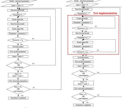
The whole BGA procedure previously described is illus-trated in Fig. 3a.

3.1 Parallelization of the Jacobian matrix evaluation The most relevant contribution to the total computational time required by the inverse procedure is ascribed to the for-ward model runs (i.e. the computation of each element in the Jacobian matrix) rather than to the bgaPEST operations. However, since each of the Np runs in Eq. (15) checks the sensitivity of the observations to the variation of a single pa-rameter, the solution of a run does not affect the other ones. Therefore, in order to reduce the computational burden, the independentNpruns can be potentially performed in parallel.

In this work, the PARFLOOD two-dimensional-GPU nu-merical model presented in Vacondio et al. (2014) and Vacondio et al. (2017) has been adopted for routing the in-flow hydrograph. Therefore, the bgaPEST routine to evalu-ate the Jacobian matrix has been parallelized in order to take advantage of the computational capability of modern high-performance computing (HPC) clusters, which are usually equipped with many GPUs. The implemented parallel pro-cedure, which is illustrated in the flow chart of Fig. 3b, han-dles the parallelism among host and GPUs by means of the Secure Shell network protocol (SSH) and manages the most operative parts of the parallelism (login, run, etc.) outside of the bgaPEST code. In the serial version (Fig. 3a), the crucial part of the Jacobian matrix evaluation consists of a DO-loop over the parameters. Considering the parameteri, the input file that will be read by the forward model is first written, then the model is run, and the resulting values are finally read. In the modified version (Fig. 3b), this main loop is split in three parts: first, the input files (equal toNp) in which a particular parameter is modified are written, then the forward model is run (Nptimes), and a second loop is finally performed to read all the resulted values.

3.2 The forward model

A. Ferrari et al.: Discharge hydrograph estimation at upstream-ungauged sections 5305

Figure 3.Illustration of BGA algorithm in the serial(a)and parallel(b)version.

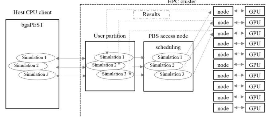
two-dimensional SWE-GPU code on the device (GPU). In the present work, a cluster with 10 NVIDIA® Tesla®P100 GPUs hosted by the University of Parma was adopted. As shown in Fig. 4, the bgaPEST algorithm runs on the CPU of a computer, where the Np simulations (assumed equal to 3 for the sake of simplicity in Fig. 4) are first created and then sent to the server user partition by means of the SSH proto-col. Here, the cluster access node schedules all the jobs sub-mitted by the users, using the HPC scheduler Portable Batch System (PBS). Then, each simulation is assigned to a spe-cific GPU node. At the end of the computation, the observa-tions are extracted and the output files remain on the cluster partition until the CPU verifies via SSH the end of the simu-lation and copies the results back. The procedure illustrated in Fig. 4 and later described represents the parallelization of the Jacobian matrix computation.

Listing 1 provides a detailed description of the “run for-ward model” shell file. In order to use the algorithm for dif-ferent test cases and potentially on difdif-ferent HPC clusters, all the paths are first declared together with the involved

Figure 4.Schematization of the data transfer assuming three parameters and thus three parallel simulations.

evaluate the Jacobian matrix simulating each of theNpruns fromtstarttotendis equal to

T =Np Np−1

1t, (16)

where 1t denotes the constant time interval between two consecutive parameters.

Conversely, the physical timeT∗required to simulate all the Np runs by restarting theith simulation from timeti−1 instead oftstartis equal to

T∗=(Np−1)1t+

Np

X

i=2

Np−(i−1)1t. (17) As pointed out by Eqs. (16)–(17) and exemplified in Fig. 5, this simple operation allows for the reaching of a relevant de-crease of the total computational time. Therefore, at line 8, the algorithm computes the time needed to restart the simu-lation.

In order to perform the simulation, the host logs in to the HPC cluster by means of the SSH protocol (line 9) and a sleep condition ensures the login procedure (line 10). Then the job is submitted to the queue of the cluster using exter-nal parameters for passing the name of the simulation folder and the time for restart (line 11); the submitted job contains the reference to the PBS queue and the link to the executable two-dimensional SWE-GPU code. At the end of the simu-lation, the water levels at the observation site are automati-cally extracted. Once the job is submitted, the SSH login is closed (line 12). After having submitted all the simulations, for each parameter (line 15), the code regularly (line 18) tests the presence of the end_file via SSH, which states the end of the simulation (line 20) and waits in case it is missing (line 25). Once the simulation is finished, the resulting ob-servations are copied back to the host client (line 28), and the folder is removed from the server (line 29).

Figure 5.Time reductionT∗/T as a function of the number of es-timable parameters (thex-axis is in logarithmic scale).

Conversely, theelsecondition (line 30) is true for the base run. The simulation folder with the input files is copied to the server (line 31), and the job is submitted (line 34). Then, the algorithm periodically verifies the end of the simulation and copies the results back to the host client (lines 39–49). It is relevant to note that the base run is performed first, whereas the otherNpruns can be performed in parallel.

4 Application of the inverse methodology to synthetic test cases

hydro-A. Ferrari et al.: Discharge hydrograph estimation at upstream-ungauged sections 5307

Listing 1.Run forward model for the parallel bgaPEST scheme.

graph that is unknown at the beginning of the process. There-fore, in this section the inflow hydrographs in two natural rivers in northern Italy are estimated, and the reference so-lutions, which are necessary in order to validate the inverse procedure, are obtained as follows (D’Oria et al., 2014). Con-sidering the domain in Fig. 6, a selected inflow discharge Qref is routed from the upstream section A to the down-stream boundary D, where a rating curve is imposed far away from C. The resulting water level hydrographs are extracted at sites B and C. The inverse procedure is then applied to the sub-domain illustrated with solid line in Fig. 6 by assuming the water levels in sites B and C (derived in step 1) as the ob-servations and downstream boundary condition, respectively. The information in sub-reach C–D is only preparatory for setting up the synthetic cases, and it is not used in the inverse procedure. Imposing a rating curve in D allows one to obtain water levels with a non-unique stage–discharge relationship in section C, which is more close to the real situations when applying the inverse procedure. The methodology estimates the inflowQestassuming that no information is available on the discharge (or water stage) at the inflow section A.

Quantitative information about the accuracy of the inverse methodology is provided by evaluating the differences be-tween the referenceQrefand the estimatedQesthydrographs by means of three different indicators. First, the Nash– Sutcliffe efficiency criterion (Nash and Sutcliffe, 1970) Eh was adopted according to the following relation;

Eh= "

1−

PNp

i=1(Qi ref_−Q

iest)2

PNp

i=1(Qi

ref_−Qref₎2 #

·100, (18)

Figure 6.Exemplification of a test case definition.

whereNpis the number of parameters,Qrefi andQesti are the

ith reference and estimated inflow values, respectively, and Qrefis the mean value of the reference hydrograph. Then, the root-mean-square error (RMSE) was evaluated as follows:

RMSE=

s PN

i=1(Qiref−Qiest)2

Np

. (19)

Finally, the estimation error in the peak dischargeEpwas assessed as

Ep= "

Qest_p

Qref p

−1 #

·100, (20)

whereQest_p andQref_p denote the peak discharge value of the estimated and reference hydrographs, respectively.

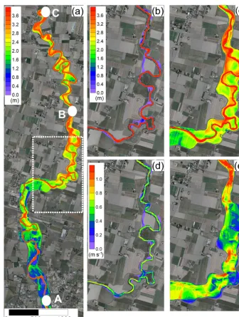
Figure 7.Map of the maximum simulated water depths for the Parma River.(a)the upstream (A) and downstream (C) boundary conditions and the intermediate observation site (B) are indicated. With reference to the area marked with dotted white line in(a),(b)and(c)represent the water depths and(d)and(e)the velocity field at low and high discharge values, respectively.

schemes not suitable to accurately describe the flood propa-gation.

The bathymetry was derived from a 1 m resolution DTM obtained through a LiDAR survey carried out in drought con-dition. The domain was discretized by means of a Cartesian grid with cell sizes 1x=1y=4 m, and about 275×103 computing cells were adopted. The Manning roughness coef-ficient was assumed equal to 0.05 s m−1/3. The steady-state values of water depth and velocity fields, obtained consid-ering the initial discharge value of the hydrograph, were adopted as initial conditions.

The inflow condition to be estimated was assumed as fol-lows (D’Oria et al., 2015);

Q(t )=A+B·f (t, b, k), (21)

wheretdenotes the time,Athe base flow (constant value),B the volume above the base flow (constant value), andf the gamma distribution, which states that

f (t, b, k)= 1

kb_0(b)t b−1_e−t

k_{, (22)}

A. Ferrari et al.: Discharge hydrograph estimation at upstream-ungauged sections 5309

parameter, respectively. The parameters of the gamma distri-bution were set as follows:A=100 m3s−1_,B=3×107_m3_, b=6, andk=10 000 s. The resulted flood wave presented a peak value of about 630 m3s−1 at time (b−1)k≈14 h (Fig. 8a).

During the estimation, when the sensitivity to the first pa-rameterp1is investigated, the steady-state flow for the ini-tial discharge is also recomputed. This means that parameter p1determines not only the first value of the estimated flood wave but also governs the initial condition of the river reach. The inflow hydrograph duration was limited to 40 h, and it was discretized using 2 h time interval (Np=21), whereas the observation stage hydrographs were discretized every 0.5 h. The prior pdf was defined by means of a Gaussian co-variance function, and the initial structural parameters were set as reported in Table 1. In order to avoid non-physical dis-charge values during the computations, non-negativity was enforced to the unknown parameters by performing the es-timation in a logarithmic space. The initial model parameter values were defined by applying the Linesearch tool of the bgaPEST, which dampens the solution between successive iterations (Fienen et al., 2013) and avoids numerical instabil-ities that may occur starting from a first choice of the param-eters too far from the true one.

The inflow hydrograph was estimated first considering true observations (the variance was set equal to 10−8m2to take into account the truncation error). Then, the same discharge hydrograph was defined corrupting the observed water lev-els with random errors uniformly distributed with maximum deviations of±0.05 m and variance 10−3m2(Fig. 8b).

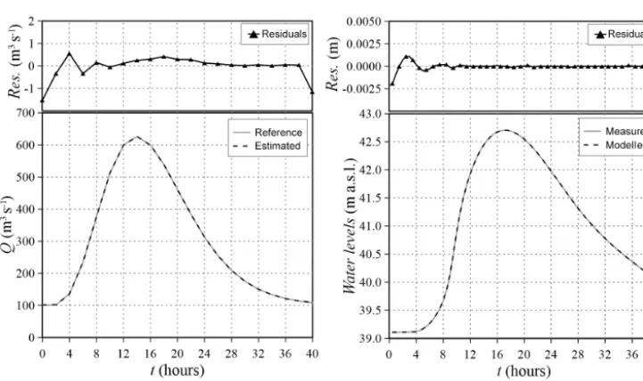
Qualitative assessment of the inverse methodology is achieved by comparing the reference with the estimated in-flow hydrograph, as well as the observed with the modelled water levels in the observation site. Considering the simula-tion without errors in the observasimula-tions, Fig. 9 shows that the estimated flood wave overlaps the reference one (a), and the modelled water levels agree almost perfectly with the mea-sured ones (b).

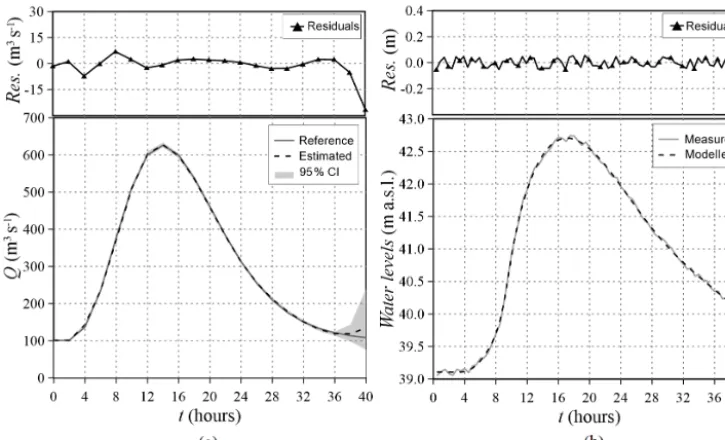
The results of the simulation with random errors corrupt-ing the observations are depicted in Fig. 10. The estimated flood wave matches well with the reference one again, pre-senting a misfit relative to the peak value lower than 5 %, and the modelled water levels similarly reproduce the reference ones with a residual of less than 1 %. Only the last value of the reconstructed flood wave is slightly overestimated, since the more the tested parameter nears the end of the wave, the fewer observations contain information about the related ef-fects, as illustrated by the increasing range of the 95 % cred-ibility interval. However, the “true” discharge values are in-side the 95 % credibility interval, thus confirming the high accuracy of the solution. In addition to this behaviour at the end of the discharge hydrograph (that can be postponed extending the hydrograph total duration), very small differ-ences between the observed and modelled variables appear when abrupt changes in the inflow function are present (e.g.

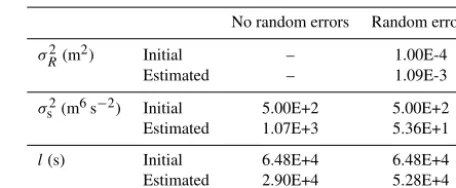
Table 1.Parma River: initial and estimated structural parameters and epistemic error variance.

No random errors Random errors

σ_R2(m2) Initial – 1.00E-4

Estimated – 1.09E-3

σs2(m6s−2) Initial 5.00E+2 5.00E+2

Estimated 1.07E+3 5.36E+1

l(s) Initial 6.48E+4 6.48E+4

Estimated 2.90E+4 5.28E+4

Table 2.Parma River: Nash–SutcliffeEh, root-mean-square error (RMSE), and error in the peak dischargeEpvalues.

Eh(–) RMSE (m3s−1) Ep(%) No random errors 99.99 0.49 −0.04 Random errors 99.88 6.65 0.15

the initial transition from the steady state to the flood wave). This behaviour is due to the regularization introduced into the solution by the prior information that imposes some degree of continuity and/or smoothness to the estimated hydrograph. However, the residuals are practically negligible, and abrupt discontinuities in the inflow hydrographs are not common in natural floods.

The structural parameters and the epistemic error variance estimated in the presence and absence of corrupted observa-tions are reported in Table 1.

An assessment of the methodology accuracy has been quantified by means of the Nash–Sutcliffe Eh, root-mean-square error (RMSE), and error in the peak dischargeEp val-ues reported in Table 2. TheEhvalues are greater than 99 %, theEpvalues are almost negligible and the RMSE is less than 0.5 m3s−1without random errors and reaches the maximum value of 6 m3s−1with corrupted observations.

Figure 8.Parma River: flow and stage hydrographs at sections A and C, respectively,(a)and observation error distribution(b).

Figure 9. Parma River: reference and estimated inflow hydrograph(a)and observed (uncorrupted) and modelled water levels(b). The residuals between reference and estimated values are also reported.

The domain was discretized by means of a non-uniform Block-Uniform Quadtree (BUQ) grid (Vacondio et al., 2017), resulting in 77×103computing cells. The Manning rough-ness coefficient in the riverbed was assumed equal to 0.05 s m−1/3(Vacondio et al., 2016).

The discharge hydrograph to be estimated is the flood wave of a 20-year return period of the Secchia River, with a peak value of about 780 m3s−1. In order to increase the non-smoothness of the wave, a quite abrupt increment that separates the initial steady-state condition (100 m3s−1) from the rising limb was introduced (Fig. 12a). It is noteworthy that this flow hydrograph is characterized by a pseudo-real irregular shape, which cannot be properly approximated by an analytical parametric function (e.g. Gamma distribution, Pearson function). The inflow hydrograph ended in 72 h and

was discretized using 2 h time interval (Np=37), whereas the observed stage hydrograph was discretized every 0.5 h. The inflow hydrograph was first estimated assuming that the true water levels extracted at section B only had a truncation error resulting in a variance of 10−8m2, and then consider-ing corrupted observations with random errors uniformly dis-tributed with maximum deviations of±0.05 m and variance of 10−3m2(Fig. 12b). Figure 12a also depicts the discharge hydrograph at the downstream boundary condition section C in order to highlight the attenuation effect exerted by the flood plains and floodable areas.

Gaus-A. Ferrari et al.: Discharge hydrograph estimation at upstream-ungauged sections 5311

Figure 10.Parma River: reference and estimated (with a 95 % credibility interval) inflow hydrographs(a)and observed (corrupted) and modelled water levels(b). The residuals between reference and estimated values are also reported.

Figure 11.Map of the water depths at the flood peak occurrence on the Secchia River, with indication of the upstream (A) and down-stream (C) boundary conditions and the intermediate observation site (B).

sian covariance function in the configuration with and with-out corrupted observations, respectively (Table 3).

As shown in Fig. 13 for the simulation without corrupted observations, the estimated flood wave matches almost per-fectly with the reference one, and the modelled water levels agree with the measured ones.

The results of the simulation with corrupted observations depicted in Fig. 14 highlight that both the shape and the peak value are well captured. The small discrepancies between the estimated peak flood wave and the reference one are

essen-Table 3.Secchia River: initial and estimated structural parameters and epistemic error variance.

No random errors Random errors

θ(m6s−3) Initial 1.00E-10 –

Estimated 3.97E-6 –

σ_R2(m2) Initial – 1.00E-4

Estimated – 1.11E-3

σs2(m6s−2) Initial – 5.00E+2

Estimated – 1.38E+1

l(s) Initial – 4.32E+4

Estimated – 3.88E+4

tially caused by the fact that the portion with the peak is dis-cretized with only a few parameters and that the adopted co-variance function smooths the solution.

The structural parameters and the epistemic error variance estimated in the presence and absence of corrupted observa-tions are reported in Table 3.

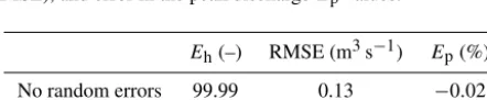
The indicators used for evaluating the accuracy of the methodology are reported in Table 4. The Nash–Sutcliffe ef-ficiencyEhvalues exceed 99 %, the errors in the peak flow Epare almost negligible, and the RMSE is less than 1 m3s−1 without random errors and reaches the maximum value of 16 m3s−1 with corrupted observations; these values high-light the accuracy of the procedure in estimating the overall shape and peak of the inflow hydrograph.

Figure 12.Secchia River: flow hydrograph in section A and flow and stage hydrographs in section C(a)and observation error distribution(b).

Figure 13.Secchia River: reference and estimated inflow hydrograph(a)and observed (uncorrupted) and modelled water levels(b). The residuals between reference and estimated values are also reported.

Table 4.Secchia River: Nash–SutcliffeEh, root-mean-square error (RMSE), and error in the peak dischargeEpvalues.

Eh(–) RMSE (m3s−1) Ep(%) No random errors 99.99 0.13 −0.02 Random errors 99.44 16.57 2.89

The computational time of the whole inflow hydrograph simulation (72 h) is 9.62 min, whereas the simulations for evaluating the Jacobian matrix and testing parameters 2– 37 required a computational time progressively lower than 9.62 min, thanks to the restart option illustrated in the Sect. 3. In order to evaluate the total time required by the inverse

Vacon-A. Ferrari et al.: Discharge hydrograph estimation at upstream-ungauged sections 5313

Figure 14.Secchia River: reference and estimated (with a 95 % credibility interval) inflow hydrograph(a)and observed (corrupted) and modelled water levels(b). The residuals between reference and estimated values are also reported.

Table 5.Secchia River: characteristics of the simulation.

Number of parametersNp 37

Physical total time of the inflow hydrograph 72 h Physical total time of the run testing the 1st parameterp1, assuming 100 h for reaching the steady state condition 172 h Computational time of the whole inflow hydrograph simulation (72 h) 9.62 min Computational time of the run testing the 1st parameter (172 h) 19.38 min Number of the BGA iterationsNifor the model parameter estimation 4 Number of the BGA iterationsNofor the structural parameter estimation 4 Total number of simulationsNt(Eq. 15) 609

dio et al. (2014) pointed out that the PARFLOOD code led to a speed-up of up to 2 orders of magnitude if compared to a serial CPU code. Therefore, if a serial BGA procedure and the GPU forward model would have required about 4 com-putational days, the inverse problem solution with a serial forward code would have ended in 400 computational days, making the use of the inverse procedure practically infeasi-ble.

5 Reconstruction of a historical event: the December 2009 flood wave on the Secchia River

The inverse procedure is now validated by investigating the December 2009 flooding event on the Secchia River, which is one of the most significant events that occurred in the last 10 years in this river. The Interregional Agency for the Po River (AIPo) monitored the river and provided the water stage hydrographs recorded in the two gauging stations indi-cated in Fig. 11 with letters B and C, respectively. As shown

in Fig. 15, the recorded water levels present more than one rising and recession limb; thus, besides the challenges related to a real field application, this test also aims at addressing the estimation of an inflow with multiple peaks. In order to es-timate the discharge in section A (Fig. 11), the water levels recorded at points B and C were assumed as observations and the downstream boundary condition, respectively. The event was simulated from 21:00 LT on 22 December 2009 to 12:00 LT on 26 December, with a total duration of 87 h. The water levels were recorded every 0.5 h, whereas the un-known inflow hydrograph was discretized into 88 parameters (one per hour,Np=88).

The studied domain is the same as the one previously adopted for a synthetic inflow; thus, the reader is kindly re-ferred to Sect. 4.2 for the information about bathymetry, ini-tial conditions, and the roughness configuration.

Figure 15.December 2009 recorded stage hydrographs on the Sec-chia River at sections B and C.

Table 6.Secchia 2009 event: initial and estimated structural param-eters.

σ_s2(m6s−2) l(s) Initial 5.00E+2 6.48E+4 Estimated 1.49E+1 3.36E+4

prior pdf was described by means of a Gaussian covariance function; the initial and estimated structural parameters are reported in Table 6.

Figure 16 shows the estimated flood wave (and the 95 % credibility interval), which presents an irregular shape and two main peaks, as it could be expected from the observed stage hydrograph. Moreover, an additional small intermedi-ate peak is captured that was not as evident in the registered water levels at section B (Fig. 15), even if a little pronounced local maximum can be seen around 15:00 LT on 24 Decem-ber 2009. The resulting flood wave presents neither instabili-ties nor oscillations. During the computation, the variance of the epistemic error was assumed equal to 10−3m2; as shown in Sect. 4, this means considering the observed water levels corrupted with random errors with maximum deviations of

±0.05 m. In Fig. 16, the flood wave estimated by increasing the variance by half an order of magnitude is also depicted (dotted line); the solution appears slightly smoothed in a few points but substantially similar when compared to the inflow resulting in the smaller variance, which is thus considered the estimated inflow of the studied event. The comparison between modelled and measured water levels at section B is presented in Fig. 17; it is relevant to note that the residuals between the two hydrographs are mostly less than 2 cm, and only in a few points of the first rising limb do they reach the highest value of 18 cm.

With the aim of validating the methodology for this real application, it is noteworthy that the upstream section of the river is located immediately downstream from a flood control reservoir equipped with water level sensors. Therefore, the “reference” discharge hydrograph has been obtained from

Figure 16.Secchia 2009 event: estimated inflow hydrographs as-suming the epistemic error variance equal to 10−3m2 and 5×

10−3m2. The 95 % credibility interval applies to the simulation with the epistemic variance equal to 10−3m2.

Figure 17.Secchia 2009 event: observed and modelled water levels in section B. The residuals between recorded and estimated values are also reported.

the dam’s geometrical data (i.e. number and dimension of the bottom openings, crest length of the spillway, etc.) and the recorded water levels adopting the classic hydraulic the-ory of sluice gates and spillways.

dif-A. Ferrari et al.: Discharge hydrograph estimation at upstream-ungauged sections 5315

Figure 18.Secchia 2009 event: comparison among the inflow hy-drographs obtained from the inverse procedure using two different Manning coefficients and the envelope of different solutions ob-tained using the records at the flood control reservoir.

ferent value in order to assess the effect of this coefficient on the solution. Particularly, the Manning coefficient, originally set to 0.05 s m−1/3, was decreased by 15 % (0.0425 s m−1/3), which, for example, can happen due to seasonal changes in vegetation. As shown in Fig. 18, the estimated flood waves are similar, and the highest difference, which is in corre-spondence with the main peak, is less than 6 %. Therefore, the influence of assuming a “wrong” roughness coefficient is less than linear in the discharge estimation. Despite all the involved approximations, this comparison confirms that the proposed inverse procedure is capable of estimating inflow hydrographs with multiple peaks and irregular shapes in real rivers.

6 Conclusions

In this work the inverse problem of estimating the unknown inflow hydrograph in an upstream-ungauged section, having water level information only in downstream sites, has been solved by means of a Bayesian methodology. The key as-pects in the solution of this problem have been the adoption of a parallel two-dimensional SWE code running on GPUs and the performance of the simulations over a HPC cluster. The parallelization of the runs useful for the Jacobian matrix computation and the implementation of an ad hoc procedure, which allows one to take advantage of any HPC cluster with GPUs, have provided a remarkable reduction of the compu-tational costs. In a test case, this parallel procedure reduced the computational time by a factor of 8 against running the two-dimensional SWE code on a single GPU. Furthermore, the analysis of the runtimes has highlighted that the use of a parallel hydraulic forward routing model is theconditio sine qua nonfor solving this type of inverse problem, whereas the adoption of a serial code would lead to inadmissible compu-tational times. The inverse procedure has been validated con-sidering two different natural rivers; in both tests, no instabil-ities due to the adopted inverse procedure or to the

availabil-ity of a stable, fast, and accurate forward hydraulic model arose. Moreover, the obtained results have highlighted that the implemented procedure estimates the unknown inflow hydrographs with different and irregular shapes and in the presence of corrupted observations well; quantitative indica-tors have proved the accuracy of the methodology. In all the presented tests, the resulting Nash–Sutcliffe efficiency cri-terion exceeded 99 %, the error in the peak discharge was less than 3 %, and the RMSE was less than 2 %. Finally, the proposed inverse procedure allowed for the estimation of a historical flood wave characterized by the presence of mul-tiple peaks, without causing instabilities in the solution. The test cases were simulated while taking advantage of the HPC cluster of the University of Parma. However, since the im-plemented procedure is general, it is possible to adopt clouds of GPUs or online mini clusters, which are now common and accessible to everyone. The adopted Bayesian software (bgaPEST) is open access, and two-dimensional SWE mod-els are a quite common tools for practitioners, even if few of them were fast enough to perform the necessary simula-tions with a reasonable computing time until now. Therefore, the 2-D coupled methodology proposed here can be adopted in the near future by professional hydrologists, too, who are involved, for example, in the design of hydraulic infrastruc-tures, as well as for engineers working on water resource management (i.e. irrigation systems, hydroelectric power sta-tions, etc.) or forensic activities. The future development of the methodology will also focus on the possibility of recon-structing the flood waves in the presence of levee breaches and flooding outside the river region, where the adoption of a two-dimensional SWE model is mandatory.

Data availability. The bgaPEST software is open source and avail-able at the link: https://pubs.usgs.gov/tm/07/c09/ (Fienen et al., 2013) The PARFLOOD model is available for non-commercial scientific collaboration upon request from Renato Vacondio ([email protected]). The recorded water levels on the Secchia River were provided by the Interregional Agency for the Po River (AIPo; https://www.agenziapo.it/, last access: 12 October 2018).

Competing interests. The authors declare that they have no conflict of interest.

Edited by: Roberto Greco

Reviewed by: Antonis D. Koussis and one anonymous referee

References

Beven, K. J.: Rainfall-runoff modelling: the primer, John Wiley & Sons, 2011.

Bruen, M. and Dooge, J. C. I.: Harmonic analysis of the stability of reverse routing in channels, Hydrol. Earth Syst. Sci., 11, 559– 568, https://doi.org/10.5194/hess-11-559-2007, 2007.

Butera, I., Tanda, M. G., and Zanini, A.: Simultaneous identifica-tion of the pollutant release history and the source locaidentifica-tion in groundwater by means of a geostatistical approach, Stoch. Env. Res. Risk A., 27, 1269–1280, 2013.

Das, A.: Reverse stream flow routing by using Muskingum models, Sadhana, 34, 483–499, 2009.

Doherty, J. E.: PEST, Model-Independent Parameter Estimation – User Manual, sixth ed., Tech. rep., Watermark Numerical Com-puting, Brisbane, Australia, 2016.

Dooge, J. and Bruen, M.: Problems in reverse routing, Acta Geo-physica Polonica, 53, 357–371, 2005.

D’Oria, M. and Tanda, M. G.: Reverse flow routing in open chan-nels: A Bayesian Geostatistical Approach, J. Hydrol., 460, 130– 135, 2012.

D’Oria, M., Mignosa, P., and Tanda, M. G.: Bayesian estimation of inflow hydrographs in ungauged sites of multiple reach systems, Advances in Water Resources, 63, 143–151, 2014.

D’Oria, M., Mignosa, P., and Tanda, M. G.: An inverse method to estimate the flow through a levee breach, Adv. Water Resour., 82, 166–175, 2015.

Eli, R., Wiggert, J., and Contractor, D.: Reverse flow routing by the implicit method, Water Resour. Res., 10, 597–600, 1974. Fienen, M., Hunt, R., Krabbenhoft, D., and Clemo, T.:

Ob-taining parsimonious hydraulic conductivity fields using head and transport observations: A Bayesian geostatistical param-eter estimation approach, Water Resour. Res., 45, W08405, https://doi.org/10.1029/2008WR007431, 2009.

Fienen, M. N., Clemo, T., and Kitanidis, P. K.: An inter-active Bayesian geostatistical inverse protocol for hy-draulic tomography, Water Resour. Res., 44, W00B01, https://doi.org/10.1029/2007WR006730, 2008.

Fienen, M. N., D’Oria, M., Doherty, J. E., and Hunt, R. J.: Approaches in highly parameterized inversion: bgaPEST, a Bayesian geostatistical approach implementation with PEST: documentation and instructions, Tech. rep., US Geological Sur-vey, available at: https://pubs.usgs.gov/tm/07/c09/ (last access: 12 October 2018), 2013.

Glickman, M. E. and Van Dyk, D. A.: Basic bayesian methods, Top-ics in BiostatistTop-ics, 319–338, 2007.

Hoeksema, R. J. and Kitanidis, P. K.: An application of the geo-statistical approach to the inverse problem in two-dimensional groundwater modeling, Water Resour. Res., 20, 1003–1020, 1984.

Kitanidis, P. K.: Quasi-linear geostatistical theory for inversing, Wa-ter Resour. Res., 31, 2411–2419, 1995.

Kitanidis, P. K. and Vomvoris, E. G.: A geostatistical approach to the inverse problem in groundwater modeling (steady state) and one-dimensional simulations, Water Resour. Res., 19, 677–690, 1983.

Koussis, A. D. and Mazi, K.: Reverse flood and pollution routing with the lag-and-route model, Hydrolog. Sci. J., 61, 1952–1966, 2016.

Koussis, A. D., Mazi, K., Lykoudis, S., and Argiriou, A. A.: Reverse flood routing with the inverted Muskingum storage routing scheme, Nat. Hazards Earth Syst. Sci., 12, 217–227, https://doi.org/10.5194/nhess-12-217-2012, 2012.

Leonhardt, G., D’Oria, M., Kleidorfer, M., and Rauch, W.: Estimat-ing inflow to a combined sewer overflow structure with storage tank in real time: evaluation of different approaches, Water Sci. Technol., 70, 1143–1151, 2014.

Michalak, A. M., Bruhwiler, L., and Tans, P. P.: A geo-statistical approach to surface flux estimation of atmo-spheric trace gases, J. Geophys. Res.-Atmos., 109, D14109, https://doi.org/10.1029/2003JD004422, 2004.

Nash, J. E. and Sutcliffe, J. V.: River flow forecasting through con-ceptual models part I – A discussion of principles, J. Hydrol., 10, 282–290, 1970.

Saghafian, B., Jannaty, M., and Ezami, N.: Inverse hydrograph rout-ing optimization model based on the kinematic wave approach, Eng. Optimiz., 47, 1031–1042, 2015.

Snodgrass, M. F. and Kitanidis, P. K.: A geostatistical approach to contaminant source identification, Water Resour. Res., 33, 537– 546, 1997.

Szymkiewicz, R.: Solution of the inverse problem for the Saint Venant equations, J. Hydrol., 147, 105–120, 1993.

Vacondio, R., Dal Palù, A., and Mignosa, P.: GPU-enhanced finite volume shallow water solver for fast flood simulations, Environ. Modell. Softw., 57, 60–75, 2014.

Vacondio, R., Aureli, F., Ferrari, A., Mignosa, P., and Dal Palù, A.: Simulation of the January 2014 flood on the Secchia River using a fast and high-resolution 2D parallel shallow-water numerical scheme, Nat. Hazards, 80, 103–125, 2016.

Vacondio, R., Dal Palù, A., Ferrari, A., Mignosa, P., Aureli, F., and Dazzi, S.: A non-uniform efficient grid type for GPU-parallel Shallow Water Equations models, Environ. Modell. Softw., 88, 119–137, 2017.