A Lack of fit Test for Econometric Applications to Cross section Data

and Labor Relations Review 31 (Oct. 1977), 45-60.

,_ "Concentration and Professional Earnings in Manu- facturing," Industrial and Labor Relations Review 31 (Apr. 1978), 379-384.

Freeman, Richard B., and James L. Medoff, "The Impact of the Percentage Organized on Union and Nonunion Wages," this REVIEW 63 (Nov. 1981), 561-572. Haworth, Charles T., and David W. Rasmussen, "Human

Capital and Inter-Industry Wages in Manufacturing," this REVIEW 53 (Nov. 1971), 376-380.

Haworth, Charles T., and Carol J. Reuther, "Industrial Con- centration and Inter-Industry Wage Determination," this REVIEW 60 (Feb. 1978), 85-95.

Hendricks, Wallace, "Unionism, Oligopoly and Rigid Wages," this REVIEW 63 (May 1981), 198-205.

Levinson, Harold M., "Unionism, Concentration and Wage Changes: Toward a Unified Theory," Industrial and Labor Relations Review 20 (Jan. 1967), 198-205. Masters, S. H., "Wages and Plant Size: An Interindustry

Analysis," this REVIEW 51 (Aug. 1969), 341-345. Mellow, Wesley, "Employer Size and Wages," this REVIEW 64

(Aug. 1982), 495-501.

Miller, Edward M., "Large Firms Are Good For Their

Workers: Manufacturing Wages as a Function of Firm Size and Concentration," The Antitrust Bulletin (Spring 1981), 145-154.

Pugel, Thomas A., "Profitability, Concentration and the In- terindustry Variation in Wages," this REVIEW 62 (May 1980), 248-253.

Rapping, Leonard A., "Monopoly Rents, Wage Rates, and Union Wage Effectiveness," Quarterly Review of Eco- nomics and Business 7 (Spring 1967), 31-47.

Ross, Stephen A., and Michael L. Wachter, "Wage Determina- tion, Inflation, and the Industrial Structure," The American Economic Review 63 (Sept. 1973), 675-692. Segal, Martin, "The Relation between Union Wage Impact

and Market Structure," Quarterly Journal of Economics 78 (Feb. 1964), 96-114.

Sparrow, Dorothy, "Changing Market Structure: Impact on Union Wage Gains," Industrial Relations 10 (May 1971), 160-167.

Stafford, Frank P., "Concentration and Labor Earnings: Com- ment," The American Economic Review 58 (Mar. 1968), 174-181.

Weiss, Leonard W., "Concentration and Labor Earnings," American Economic Review 56 (Mar. 1966), 96-117.

A LACK-OF-FIT TEST FOR ECONOMETRIC APPLICATIONS

TO CROSS-SECTION DATA

Howard E. Doran and Jan Kmenta*

experimental statisticians but mostly unknown to econometri- cians is presented. The test is applicable in situations in which there are replicated observations on the dependent variable. In this paper the test is modified to allow for heteroskedasticity usually encountered when dealing with cross-sectional observa- tions, and illustrated by an application to an earnings function estimated from a sample survey of Norwegian women.

I. Introduction

The lack-of-fit (LOF) test is a model specification test that can be applied when there are replicated observa- tions on the dependent variable corresponding to ob- servations on the explanatory variables. Basically, the test utilizes the additional information that comes from

within-group variation. As the situation of replicated observations is normal in experimental work, the test is well known to experimental statisticians but appears to be almost unknown to econometricians. (A survey of econometric text books has revealed no mention of the test.) This is probably due to the strong emphasis in econometrics on the methodology applicable to time- series data involving a single observation on the depen- dent variable for each set of observed values of the explanatory variables. By contrast, when cross-sectional data are used, there can be many units (individuals, firms, families) that are characterized by the same val- ues of explanatory variables (e.g., incomes, prices, edu- cational levels). In this situation a lack-of-fit test could often be profitably applied as an aid to appropriate model specification.

The main purpose of the paper is to draw the atten- tion of econometricians to the possibilities offered by the lack-of-fit test (see also Battese (1977)). The paper is organized as follows. Section II contains a development and an explanation of the test. In section III the test is generalized to allow for heteroskedasticity which fre- quently characterizes relations pertaining to cross-sec- tional observations. Finally, in section IV the test is applied to the standard semilog earnings function due to Mincer (1974), utilizing data from the Norwegian Fertility Survey of 1977.

Received for publication September 24, 1984. Revision accepted for publication June 10, 1985.

* University of New England, Australia, and University of Michigan, respectively.

A major part of this work was done while the authors were Fellows of the Alexander von Humboldt Foundation at the University of Bonn, Germany. Comments by Michael McAleer, Saul Hymans, Karl Lin, Jerry Thursby, G. S. Maddala and by the anonymous referees are gratefully acknowledged. Special thanks are due to Helge Brunborg and the Norwegian Central Bureau of Statistics for providing the survey data used in this paper, and to Jeffrey Pliskin who was very helpful with sugges- tions and who carried out all of the computer work involved.

II. The Lack-of-Fit Test

Suppose that an n x 1 random vector Y is normally distributed with mean ,u and covariance matrix a2I.

The null hypothesis specifies a linear model of the form

y = Xf, (1)

where X and /B are n X K and K

x

,u=X +3Zy, (2)

where Z is a matrix of values of unspecified omitted explanatory variables (including possibly higher powers of X) of dimension n X L (L < m - K) such that Z'X * 0, and -y * 0. Note that we assume that if the model is misspecified, there are m distinct observations on X and Z (although those on Z are not measured because they are not known), and that for each such observation there are ni observations on the dependent variable Y. That is, under Ho we have

Yij = x,,8 + uij (i = 1,

m;

ni)

y= x,f + z,y _{+ uij}

where xi and zi represent the i th _{row of X and Z,}

respectively.' Both variables X and Z are considered to be fixed in repeated samples.

The error sum of squares (SSE) from the regression of Y on X is given by

m n,

SSE=>

E(y-

Yj2

i=1 j=1

where Y, denotes the jth _{observation on the dependent}

variable in the ith _{group. As the} ith _{group observations}

are all characterized by the same observation on the explanatory variables, the fitted values

_Yl

Y% - Y

y.i= yo

and it follows that

m n,

SS= [(tyY e + (Y-)2

i=1 j=1

m n, m

E=1 E=1 i) + E ni(=1 y)

i=l j=l i=l

where YI is a sample mean of the ith group. Thus the error sum of squares can be partitioned into two com- ponents

m n,

SSP=

2

and

m

SSL= n(y _

A

)2

i=1

The first of these components represents the "within- group" variation which, following the experimental literature, we call the "pure error sum of squares" (SSP). The second component is termed the "lack-of-fit sum of squares" (SSL). It is the error sum of squares that would be obtained if each group were replaced by its sample mean and these sample means regressed on the same regressor variables with each observation weighted by . Defining

1n,

Si= (n -1) j ) (6)

we may write

m

SSP = (n, - 1) S2 (7) i=1

and SSP/(n - m) is seen to be a weighted average of m different estimates s7 of a2. This means that we have

two different estimators of a2, SSE/(n - K) and SSP/(n - _{m). Under Ho}

E[SSE/(n - K)] = E[SSP/(n - m)] = _a2

whereas under HA

E[SSE/(n - _{K)] > E[SSP/(n} - _{m)] = a2,}

since variation around any point other than the mean always exceeds the variation around the mean. This provides the basis for the lack-of-fit test.2

Now, under Ho

SSE/2

(8)

and

SSP/ X2 ( 9)

Further, it can easily be shown that SSL(= SSE -

SSP) and

SSP

SSL/o2

and, therefore, if the model is correctly specified,

F

SSL/( m

K)

distribution of the test statistic in (11) is unchanged under Ho and the test is still valid, but the power of the test is adversely affected. In this situation the test is in the class of the Gold- feld-Quandt test when used as a specification error test. We are indebted to Jerry Thursby for a lengthy comment c n this point.

2 _{The paper is directed to situations in which all primary}

A simple way of calculating

SSP

Y,= _I l D1j + p 2D2j + *- +AmDmj + u11 (12) where

DI= 1 for all observations in the ith group, = 0 otherwise.

Thus SSE defined in (3) represents a constrained (by the null hypothesis) error sum of squares whereas SSP represents an unconstrained error sum of squares. The F-statistic in (11) can equivalently be written as

(SSE - SSP)/(m - K)

SSP/(n-m) (

Finally, using the well-known result that F(1) v(2)

approaches X'(1l/v(l) as v(2) -- oo, we see that as

n - _{oo, SSL/a is asymptotically distributed as x2 -k}

In general, a2 is, of course, unknown. However, if G2

were known, a more powerful test would be obtained by using the chi-square result (10) rather than (11) or (13). This remark has relevance to the following section.

III. The Lack-of-Fit Test Under Heteroskedasticity

As mentioned in the introduction, the main area of usefulness in econometrics of the lack-of-fit test is in the analysis of cross-sectional data. In this context the underlying assumption that E[(Y - ,)(Y - ,u)'] = g2In

is unlikely to be realistic. We will generalize it by assuming that

E[(Y - )(Y -) ] = (14)

where

1 = diag( alI,,(1), 02n2 (2),. ,O rIn(m))

and the o,2 _{are known. Then, defining}

D

it follows that

D - Iy _{~ N( D- 'Al, In)}

and the linear specification on the mean under the null hypothesis takes the form

D- 1 _(D-1X)fP. (15)

Thus, provided the analysis is carried out in terms of the weighted observations _Yj/o, and X/ai (i = 1, 2,..., im), the test described in the previous section

follows through with one difference, namely, that o2 is

known to be equal to unity. Thus by (10), if the model is correctly specified,

SSL* X z-K (

16)

where we have used SSL* to emphasize that weighted observations are used.

In practice the q2 are rarely known and have to be

estimated. Provided the values of the omitted variables remain unchanged whenever the values of the included variables are unchanged (i.e., provided the model under HAis Yj = x,f3 + ziy + uij), the estimators s2 defined

in (6) are consistent estimators of the _uj2. These estima- tors are completely independent of the specification ,u= X,8. Thus the result in (16) is to be regarded as a large sample result; if the observations are weighted inversely by s,, then as ni -- _{oo, the distribution of}

SSL* is given by (16).

It is commonly assumed in econometrics that the variances a,2 can be related to a single variable w, through a relationship of the form

aq2 = aw ,' (w, > 0), (17)

where a and 8 are unknown parameters. Typically, w, would be a member of the regressor set, but this need not be the case. If such a model is appropriate and m > 2, then there will be gains in asymptotic efficiency if we make use of the information given in (17). A simple method of using (17) proceeds as follows. Defin- ing s5 as in (6), we have

_(n, n _-1)s2 2 2

V, = 2 Xn(i)-l'

Therefore, given that a2 = aw8,

ln

ln

+

u,

lnv,

_ln(

Bartlett and Kendall (1946) have shown that for large

n,, I( n, - 2) u, is approximately normally distributed with mean zero and variance 2. Furthermore, they showed that this approximation is likely to be good for

n, as small as 10.

Thus least squares regression of ,/( n, -2) ln S2 on (n, - _{2) and yf(n,} - 2) ln w, will produce consistent and asymptotically efficient estimates of a and 8.

IV. An Illustrative Application of the LOF Test to an Earnings Function for Women

To illustrate the use of the LOF test, we consider the effect of schooling on earnings, and in particular how this effect applies to women whose work history typi- cally differs from that of men. The standard model of earnings proposed by Mincer (1974) and frequently used in applied labor economics-most recently by Behrman and Birdsall (1983) and by Chiswick (1983)-is basically of the form:

where

W, is the wage-rate of the jth individual in the ith

group;

X, is the "on-job" work experience (common to all individuals in the i th group);

S, is the number of years of schooling (common to all individuals in the ith group);

and u,, is an independently distributed stochastic dis- turbance. (The subscripts have been adapted to the replicated data case considered by us.) Other variables, such as presence of children or headship of family, that are frequently controlled for in applied work can be subsumed under the omitted Z variables.

At least two types of possible misspecifications of equation (19) have been discussed in the literature.3 First, a study by Mincer and Polachek (1974) provides some evidence that the marginal effect of schooling on the wage-rate of people of equal work experience is not constant for women with families. A similar conclusion with respect to heads of households (of any sex) has been reached by Ryder, Stafford, and Stephan (1976) on the basis of a model of life-cycle decision making with leisure as a choice variable. This suggests the possibility of an incorrect functional form of the equation. Second, it is by no means certain that the model in (19) contains all relevant explanatory variables. In particular, Griliches (1977) contends that models such as that in (19) suffer from the fact that individual ability-likely to be correlated with schooling-has been left out. The LOF test can certainly be effective in detecting incorrect functional form since the omitted variables are now represented (at least approximately) by higher powers of X. As for the omitted "ability" variable, for the test to work well it would have to be true that all individuals of given experience and schooling are characterized by nearly the same ability, otherwise the test will lose some power.4

The preceding discussion leads to the conclusion that it may be worthwhile to apply the LOF test not only to equation (19)-to be labeled Model 1-but also to an equation that allows for a nonlinear effect of schooling as in

ln W,=

f

I

(20)

which we label Model 2. To carry out the test we used the data on about 2,000 married women taking part in

the Fertility Survey 1977 carried out by the Norwegian Central Bureau of Statistics. The survey involved a random sample of about 4,000 women but this number was reduced to about one-half after eliminating all observations that were incomplete or that corresponded to a small number of replications. Actually, all that is (theoretically) required is that n, > 1 for at least one group. The only problem with this arises under hetero- skedasticity when ai is not known and has to be esti- mated since this is impossible when n, = 1. However, if we make the assumption spelled out in equation (17) above, namely that

a2 = _awI,

then we can use those groups for which ni > K to estimate a and 8. Having found a and ,B, we obtain

"2 W 3

which can be applied to all groups. From this stage on, all groups are used and no information is thrown away. We did not pursue this refinement because our main purpose was just to illustrate the use of the LOF test. The elimination of the groups with a small number of replications may affect the substantive interpretation-if not the validity-of our results.

With respect to measurement of the variables in- volved, the following applied. Wages were measured by Kroner per hour; they are represented by actual wages for working women and by potential wages for women who did not work at the time of the interview.5 Experi- ence was measured by the number of years worked since completing the highest education. Finally, educa- tion was measured by years of schooling.6

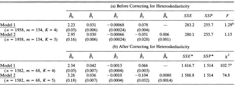
The results for both models are presented in table 1. Part (a) of the table contains the results before cor- recting for heteroskedasticity whereas part (b) shows the results after heteroskedasticity has been corrected for. The details of the correction are as follows. By reference to the large-sample procedure described in section III, we postulate that heteroskedasticity in the earnings equation takes the form

a2 = _aS," (21)

and obtain the following estimates:

a = 0.429 8 = -0.610 (F= 15.52*).

(0.173) (0.112)

(*Significant at the 1% level.) Correction for hetero- skedasticity was then implemented in accordance with equation (15).

'Along with other applied research workers, we do not address the problem of a simultaneous equation bias that may arise from the endogeneity of schooling-a point discussed at length by Griliches (1977).

4 _{See footnote 1 above. Griliches (1977) refers to "ability" as}

"an unobserved latent variable that both drives people to get relatively more schooling and earn more income, given school- ing. .." (p. 7).

5Potential wage was measured by the answer given to the question "If you were to be working just now, how much would you be paid per hour?"

6 When applying the LOF test to model 2 we also used

TABLE 1.-REGRESSION RESULTS AND LACK-OF-FIT COMPUTATIONS FOR MODELS 1 AND 2 (a) Before Correcting for Heteroskedasticity

/0 #I /2 /3 34 SSE SSP F

Model 1 2.23 0.031 -0.00068 0.078 - 283.2 255.7 1.29b

(n = 1958, m = 154, K = 4) (0.05) (0.006) (0.00024) (0.004)

Model 2 2.95 0.030 -0.00066 -0.051 0.006 280.1 255.7 1.15

(n = 1958, m = 154, K = 5) (0.16) (0.006) (0.00024) (0.028) (0.001)

(b) After Correcting for Heteroskedasticity

/30 P1 P2 /3 /4 SSE* SSP* x2

Model 1 2.34 0.042 -0.0013 0.066 -- 1 616.7 1 514 102.7a

(n = 1582, m = 68, K = 4) (0.05) (0.007) (0.0004) (0.003)

Model 2 3.26 0.036 -0.0010 -0.104 0.0080 1 588.8 1 514 74.8

(n = 1582, m = 68, K = 5) (0.18) (0.007) (0.0004) (0.032) (0.0014)

Note: Standard errors are in parentheses. a _{Significant at the 5% level.}

b Significant at the 1% level.

The most important result of table 1 is that Model 1 is rejected by the LOF test whereas Model 2 passes the test. This holds whether a correction for heteroskedas- ticity is carried out or not. Thus the evidence of Mincer and Polachek (1974) is confirmed by our results. The linear form of schooling in the earnings equation for married women appears to be inappropriate according to our evidence.7

We conclude by giving a more detailed consideration to the marginal effect of schooling on the earnings of women. Using the results for Model 2 after correcting for heteroskedasticity, we estimate the marginal effect of schooling as

[aE(n

_']

-0.104 + 0.016S,. (22)

[

as,

This result is consistent with that of Mincer and Polachek (1974) in that the effect of schooling is an increasing function of schooling. In addition, the margi- nal effect of schooling is positive for S, 2 6.5 years. As there are at least 8 years of compulsory primary school-

ing, these data suggest that the marginal effect of schooling (for fixed experience) is positive. This is con- sistent with the result which has been found for men.

7 _{It is, of course, possible that the term}

_S72

REFERENCES

Bartlett, M. S., and D. G. Kendall, "The Statistical Analysis of Variance Heterogeneity and the Logarithmic Transfor- mation," Journal of the Royal Statistical Society, Series B, 8 (1946), 128-138.

Battese, George E., "Agricultural Economists, Response Func- tions and Lack-of-fit tests," Review of Marketing and Agricultural Economics 45 (1977), 85-94.

Behrman, Jere R., and Nancy Birdsall, The Quality of School- ing: Quantity Alone Is Misleading, American Economic Review 73 (Dec. 1983), 928-946.

Central Bureau of Statistics of Norway, 1981, Fertility survey 1977 (Oslo) (1981).

Chiswick, Carmel U., Analysis of Earnings from Household Enterprises: Methodology and Application to Thailand, this REVIEW 65 (Nov. 1983), 658-662.

Griliches, Zvi, "Estimating the Returns to Schooling: Some Econometric Problems," Econometrica 45 (Jan. 1977), 1-22.

Mincer, Jacob, Schooling, Experience and Earnings (New York: Columbia University Press, 1974).

Mincer, Jacob, and Solomon Polachek, "Family Investments in Human Capital: Earnings of Women," Journal of Political Economy 82 (Mar./Apr. 1974), 76-108. Ryder, Harl E., Frank P. Stafford and Paula E. Stephan,