Bus Driving Cycle Construct Based on Principal Component Analysis for Lanzhou City

14th International Conference on Wireless Communications, Networking and Mobile Computing (WiCOM 2018) ISBN: 978-1-60595-578-0

Bus Driving Cycle Construct Based on Principal Component

Analysis for Lanzhou City

Yifan Ji, Cuiran Li, Jianli Xie, Yang Wang and Wenqian Guo

ABSTRACT

The construction of city bus driving cycle is the key to improve traffic efficiency and transportation capacity. In this paper, the data acquisition parameter model is established by taking the Lanzhou city as an example. The data collected from the vehicle recorder are divided into several kinematics sequences. The eigenvalues of these sequences are investigated by principal component analysis and cluster analysis with SPSS tool. Based on the correlation coefficient of collected data from five typical bus lines for more than one month, three representative kinematic sequences are selected to construct the bus driving cycle for Lanzhou city. Experiments show that: 1) The bus driving cycle for Lanzhou city has the characteristics of less uniform time, low average speed and frequent acceleration and deceleration; 2) There exist large differences in bus driving characteristics between the European ECE15 driving cycle, commonly used in the China's urban roads and that of Lanzhou city.

Key words: Driving conditions; Data acquisition; Principal component analysis; Cluster analysis1

1. INTRODUCTION

The vehicle driving cycle mainly describes the time velocity curve of vehicle running state. It reflects the speed change rules of vehicles in specific sections. Recently, domestic researchers have conducted in-depth research on driving cycle of some cities in China. In [1], the typical road in Hefei is taken as an example to construct road driving cycle. In [2], the driving cycle of passenger cars of Shenzhen urban area is constructed by short travel analysis. In [3], the multi wavelet decomposition algorithm of discrete wavelet transform is used to reconstruct data to establish road driving condition in Hefei. In [4], the typical driving cycle of Jinan bus are constructed by clustering analysis and Markov chain, and the effectiveness of the proposed method is verified by comparing with the measured data. In [5], the fuzzy c-means(FCM) clustering method is improved by self-organizing map(SOM) network to construct the road driving cycle in Hefei. In [6], the test data are processed by fuzzy clustering method, and the driving cycle of Xi'an urban area which can reflect the traffic flow condition is established.

This paper collects a lot of driving sample data of Lanzhou No. 137 bus and divide it into several kinematic fragments sequences. Data were processed and classified by principal component analysis and cluster analysis. Finally, three representative kinematic segments are selected to construct the bus driving cycle in Lanzhou.

2. PREPARATION FOR DRIVING CYCLE CONSTRUCTION

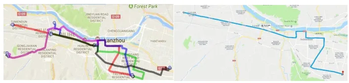
The construction of driving cycle is inseparable from data collection, and the accuracy of data acquisition is affected by test methods and test routes.

Figure 1. Road map of five typical lines Figure 2. Route map of the No.137 bus.

A. Text Planning

Considering that the test is to collect the driving data of Lanzhou bus, and the running time, running route, even the running speed of the bus have certain requirements. The test chooses the autonomous driving method to obtain bus travel sample data, that is, allowing the bus drivers to drive their bus under normal operation conditions.

The test data of five typical lines in Lanzhou are collected for more than one month. Among them, No.137 bus run through busy streets, suburban areas and ordinary streets, the proportion of its main roads and slip roads is close to the overall proportion of Lanzhou, which is more representative. Therefore, the No.137 bus is taken as an example to construct the driving cycle. The five typical routes are shown in Figure. 1. No. 137 bus routes as shown in Figure 2.

B. Data Collection

There are many driving parameters that can be collected during the actual operation, such as speed, engine speed, time, mileage, atmospheric pressure, even including environmental temperature. For the construction of bus driving cycle of Lanzhou city, the parameters of vehicle speed, engine speed and time are mainly used.

The sampling frequency of vehicle recorder used in the test is 1Hz.The sampling time is from 6:30 to 20:20.The test records the driving condition of No.137 bus for Twenty-five days and collects 313765 effective speed information.

3.DATA ANALYSIS

In this section, we divide the test data into several kinematic sequences by the principal component analysis and cluster analysis.

A. Kinematic Sequences

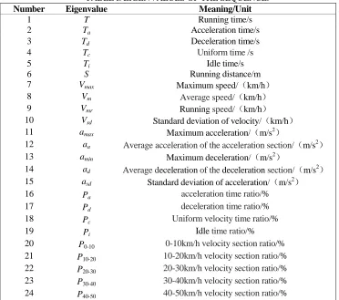
of 300s-500s kinematic sequences, each of which starts from idle point and stops at an idle point between 300s and 500s.As shown in Table I, twenty-four eigenvalues will be used to describe these kinematic fragments and the first fifteen are used for principal component analysis.

TABLE I. EIGENVALUES OF THE SEQUENCE.

Number Eigenvalue Meaning/Unit

1 T Running time/s

2 Ta Acceleration time/s

3 Td Deceleration time/s

4 Tc Uniform time /s

5 Ti Idle time/s

6 S Running distance/m

7 Vmax Maximum speed/（km/h）

8 Vm Average speed/（km/h）

9 Vmr Running speed/（km/h）

10 Vsd Standard deviation of velocity/（km/h）

11 amax Maximum acceleration/（m/s2）

12 aa Average acceleration of the acceleration section/（m/s2）

13 amin Maximum deceleration/（m/s2）

14 ad Average deceleration of the deceleration section/（m/s2）

15 asd Standard deviation of acceleration/（m/s2）

16 Pa acceleration time ratio/%

17 Pd deceleration time ratio/%

18 Pc Uniform velocity time ratio/%

19 Pi Idle time ratio/%

20 P0-10 0-10km/h velocity section ratio/%

21 P10-20 10-20km/h velocity section ratio/%

22 P20-30 20-30km/h velocity section ratio/%

23 P30-40 30-40km/h velocity section ratio/%

24 P40-50 40-50km/h velocity section ratio/%

In data processing, the following criteria are used to determine acceleration, deceleration, uniform speed and idle speed[7]:Acceleration refers to the continuous process of vehicle acceleration a≥0.1 m/s2. Deceleration refers to the continuous process of vehicle acceleration a≤-0.1 m/s2. Uniform speed refers to the continuous process of the absolute value of the vehicle acceleration |a|<0.1 m/s2. Idle speed refers to the continuous process of engine speed greater than 0 and Vmr =0

B. Principal Component Analysis

However, the actual meaning of each eigenvalues is different, the form of expression is different, and the effect of each eigenvalue on the evaluation system is also inconsistent. Therefore, we need to standardize the data processing first [8]. By means of Z normalization method, the mean value of the variables is 0 and the standard deviation is 1 after dimensionless, and the matrix expression of eigenvalues is:

11 12 1

21 22 2

1 2

=

n

n

m m mn

x x x

x x x

x x x

           

X (1)

Where xij(i=1,2,…,m;j=1,2,…,n) is the jth eigenvalue for the ith kinematic

sequence. Matrix X is normalized to get matrix Z.

11 12 1

21 22 2

1 2

=

n

n

m m mn

z z z

z z z

z z z

           

Z (2)

Where: ij j ij j x x z s 

 (3)

1 1 = m j ij i x x

m



(4)





S x x

m 

 





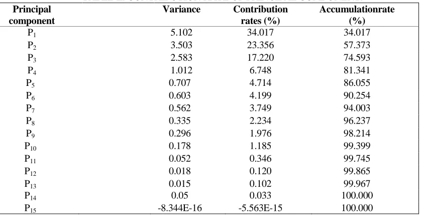
TABLE II. CONTRIBUTION RATE OF PRINCIPAL COMPONENT.

Principal component

Variance Contribution rates (%)

Accumulationrate (%)

P1 5.102 34.017 34.017

P2 3.503 23.356 57.373

P3 2.583 17.220 74.593

P4 1.012 6.748 81.341

P5 0.707 4.714 86.055

P6 0.603 4.199 90.254

P7 0.562 3.749 94.003

P8 0.335 2.234 96.237

P9 0.296 1.976 98.214

P10 0.178 1.185 99.399

P11 0.052 0.346 99.745

P12 0.018 0.120 99.865

P13 0.015 0.102 99.967

P14 0.05 0.033 100.000

TABLE III. THE CORRELATION COEFFICIENT TABLE.

eigenvalue P1 P2 P3 P4

T 0.831 0.230 -0.490 0.112

Ta 0.821 0.245 -0.366 0.056

Td 0.743 0.216 -0.521 0.021

Tc 0.800 -0.119 -0.279 -0.163

Ti -0.033 0.521 -0.377 0.633

S 0.978 0.031 -0.015 -0.025

Vmax 0.525 0.287 0.588 0.111

Vm 0.726 -0.185 0.592 -0.153

Vmr 0.655 -0.078 0.677 0.038

Vsd 0.322 0.383 0.677 0.367

amax 0.084 0.688 -0.047 -0.416

aa -0.370 0.772 -0.066 0.088

amin -0.046 -0.672 -0.028 0.395

ad 0.243 -0.680 -0.283 -0.121

asd -0.219 0.896 0.137 -0.210

Principal component analysis of data after normalization is shown in Table II. Table II shows that the accumulation rate of the first four principal components reaches 81.341%, which means that the first four principal components namely P1 P2

P3 P4, can represent data characteristics[9].The correlation coefficients of the first four

principal components and the fifteen eigenvalues are shown in Table III. The analysis can be obtained from Table III: (1) P1 mainly reflects T, Ta, Td, Tc, S, Vm, ad. (2) P2

mainly reflects amax, aa, asd. (3)P3 mainly reflects Vmax, Vmr, Vsd. (4) P4 mainly reflects

Ti, amin.

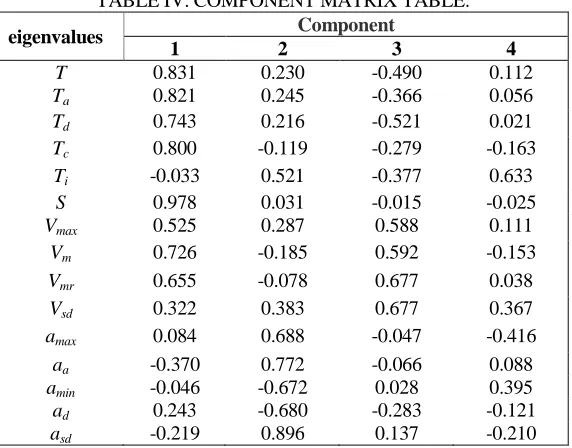
In order to classify the kinematic sequences by cluster analysis, we need to get the score of these sequences on the first four principal components. The formula for the principal component score of each kinematics sequences:

TABLE IV. COMPONENT MATRIX TABLE.

eigenvalues Component

1 2 3 4

T 0.831 0.230 -0.490 0.112

Ta 0.821 0.245 -0.366 0.056

Td 0.743 0.216 -0.521 0.021

Tc 0.800 -0.119 -0.279 -0.163

Ti -0.033 0.521 -0.377 0.633

S 0.978 0.031 -0.015 -0.025

Vmax 0.525 0.287 0.588 0.111

Vm 0.726 -0.185 0.592 -0.153

Vmr 0.655 -0.078 0.677 0.038

Vsd 0.322 0.383 0.677 0.367

amax 0.084 0.688 -0.047 -0.416

aa -0.370 0.772 -0.066 0.088

amin -0.046 -0.672 0.028 0.395

ad 0.243 -0.680 -0.283 -0.121

TABLE V. SCORE TABLE OF THE MAIN COMPONENTS.

sequences P1 P2 P3 P4

1 2.9290 -0.8669 1.0503 0.1548

2 3.92767 -2.9773 1.4788 0.0853

3 _{1.9865 -1.6979 1.8866 0.1323}

4 -0.1798 -1.5295 1.4863 0.3408

5 2.9760 3.4329 -0.7040 0.3445

6 2.9168 0.4312 -2.0797 1.1224

7 -0.5962 1.2989 1.6196 1.5895

8 3.1237 0.6764 -1.2512 -0.2821

9 2.5690 -0.4719 -3.1425 0.0005

10 3.7757 3.5250 -2.3081 0.3106

… … … … …

382 2.2072 -1.4631 0.4511 1.1699

j j

F = Ze j1, 2, ,k (7)

Where Z is the normalized data matrix, and K is the number of the principal component. The formula of the ej is:

= ij j

j

b e

 (8)

Where bij is the value of each principal component in the component matrix table, as shown in Table IV. λj is the variance of the principal component of the jth in Table II. The principal component of each kinematics sequences is shown in Table V.

C. CLUSTER ANALYSIS

Cluster analysis is a statistical method for classifying complex research objects. The purpose is to classify similar data in complex data into one class[10]. In this paper, fast clustering method (K means clustering) is used to cluster all kinematics sequences, and the motion intervals of the same traffic characteristic values are divided into one class.

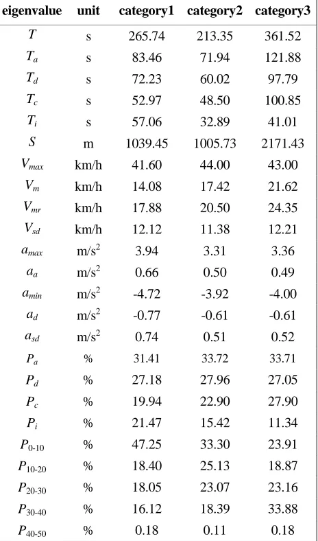
In the actual situation, according to the bus driving condition, all the kinematics sequences are clustered into three types, which are high speed, middle speed and low speed. According to the contribution rate of principal components, the first four principal components scores of kinematic sequences are selected for analysis. Table VI shows integrated eigenvalue of different categories.

24.35km/h, running distance is 2171.43m, and 30~40km/h speed segment has the highest proportion, which is 33.88%.

TABLE VI. THE COMPREHENSIVE EIGENVALUE OF THE SEQUENCE.

eigenvalue unit category1 category2 category3

T s 265.74 213.35 361.52

Ta s 83.46 71.94 121.88

Td s 72.23 60.02 97.79

Tc s 52.97 48.50 100.85

Ti s 57.06 32.89 41.01

S m 1039.45 1005.73 2171.43

Vmax km/h 41.60 44.00 43.00

Vm km/h 14.08 17.42 21.62

Vmr km/h 17.88 20.50 24.35

Vsd km/h 12.12 11.38 12.21

amax m/s2 3.94 3.31 3.36

aa m/s2 0.66 0.50 0.49

amin m/s2 -4.72 -3.92 -4.00

ad m/s2 -0.77 -0.61 -0.61

asd m/s2 0.74 0.51 0.52

Pa % 31.41 33.72 33.71

Pd % 27.18 27.96 27.05

Pc % 19.94 22.90 27.90

Pi % 21.47 15.42 11.34

P0-10 % 47.25 33.30 23.91

P10-20 % 18.40 25.13 18.87

P20-30 % 18.05 23.07 23.16

P30-40 % 16.12 18.39 33.88

P40-50 % 0.18 0.11 0.18

4. CONSTRUCTION AND ANALYSIS OF DRIVING CYCLE

Table VII shows that the average speed of buses in Lanzhou is quite close to that of Beijing, Tianjin and Shanghai[12], but the acceleration and deceleration are more frequent. The driving cycle abroad are quite different from those of Lanzhou: The ratio of acceleration and deceleration of ECE15 and Japan10 is much lower than that of Lanzhou, and the idling ratio is obviously higher. The acceleration and deceleration ratio of FTP75 is close to that of Lanzhou, but the average speed is much higher than that of Lanzhou. At present, ECE15 driving cycle are widely used in our country. Compared with the bus driving cycle for Lanzhou, the acceleration ratio is 12% lower and the idle speed ratio is 13% higher. Obviously, ECE15 driving cycle is not suitable for evaluating the driving cycle of Lanzhou bus. According to the study of this paper, the running speed of bus driving cycle for Lanzhou in Peak time is about 14km/h, the normal time is about 17km/h, and the idle time is 21km/h. It has the characteristics of short uniform time and frequent acceleration and deceleration, which is different from other cities in China. Therefore, it is quite necessary to formulate corresponding bus driving cycle for the specific conditions of bus operation in Lanzhou.

Figure 3. Proportion of time of 3 types of traffic conditions.

Figure 4. Bus driving cycle.

0% 20% 40% 60%

Low speed Medium speed High speed

-10 0 10 20 30 40 50

0 200 400 600 800 1000 1200

s

p

e

e

d

(

k

m

/h

)

0.00% 5.00% 10.00% 15.00% 20.00% 25.00% 30.00% 35.00%

0-10km/h 10-20km/h 20-30km/h 30-40km/h 40-50km/h

Figure 5. The proportion of each speed section of Lanzhou bus.

TABLE VII. COMPARISIONTABLEOFDRIVINGCYCLE IN SOME CITIES.

Region Acceleration ratio (%)

Deceleration ratio (%)

Uniform ratio (%)

Idle ratio (%)

Average speed (km/h)

Lanzhou 33.36 27.14 22.18 17.31 17.47

Tianjin 26.88 27.64 14.34 22.18 18.94

Shanghai 22.83 30.85 27.34 16.52 19.98

Beijing 25.29 30.85 27.34 16.52 19.98

ECE15 21.57 18.49 29.27 30.68 18.7

FTP75 33.4 28.88 19.55 18.01 34.07

Japan10 24.44 12.19 23.7 26.67 17.1

5. CONCLUSION

In this paper, the driving data of five typical lines of Lanzhou bus are collected by vehicle recorder, and the No.137 bus is taken as an example to analyze and construct the bus driving cycle for Lanzhou city. The results show that the bus driving cycle for Lanzhou city has the characteristics of short uniform time and frequent acceleration and deceleration, which is different from the domestic and foreign countries. The construction of the bus driving cycle can also provide a theoretical basis for the future formulation of Lanzhou bus operation plan and the choice of buses.

ACKNOWLEDGMENT

This work is partially supported by the National Natural Science Foundation of China (61661025, 61661026), and Foundation of A hundred Youth Talents Training Program of Lanzhou Jiaotong University.

REFERENCES

1. Shi Q, Zheng Y, Jiang P. 2011. “A Research on Driving Cycle of City Roads Based on Microtrips,” Automotive Engineering, 2011, 33(3): 256-261.

2. Wan X, Huang W, Qiang M. 2016. “Construction of driving cycle for passenger vehicles in Shenzhen,” Journal of Shenzhen University Science and Engineering, 33(3): 281-287.

3. Jiang P, Shi Q, Chen W. 2011. “Research on the Construction of City Road Driving Cycle Based on Wavelet Analysis,” Automotive Engineering, 33(1): 70-73+51.

5. Shi Q, Ma H, Ding J, et al.2014. “An Improved FCM Clustering Algorithm and Its Applications of Vehicle Driving Cycle Construction,” China Mechanical Engineering, 25(10): 1381-1387.

6. Lin H, Yu Q. 2015. “Construction of Sedan’s Driving Cycle in Xi’an City Based on Fuzzy Clustering,” Journal of Zhengzhou University (Engineering Science), 36(4): 96-99.

7. Zhu J, Shi Q, Zhou J. 2011 “The city bus driving cycle construction,” Technology & Economy in Areas of Communications: 2687-2690.

8. Yi Y, Chen J, Zheng R. 2017. “Game Research on Selection and Competition for Franchisees Based on Dimensionless,” Journal of Lanzhou Jiao Tong University, 6(2):63-67.

9. Zhang F. Study on Driving Cycles of City Vehicle. Wuhan University of Technology, 2005. 10. Yang Y, Yao X, Yang J. et al. 2013 “Thermo-Drifting Error Modeling of Spindle Based on

Combination of Principal Component Analysis and BP Neural Network,” Journal of Shanghai Jiao Tong University, 47(5):750-753.

11. Andre M. 1996 “Driving Cycles Development: Characterization of the Methods,”Sae Technical Papers.