by
Kelly Cooper Younge
A dissertation submitted in partial fulfillment of the requirements for the degree of
Doctor of Philosophy (Physics)
in The University of Michigan 2010
Doctoral Committee:
Professor Georg A. Raithel, Chair Professor Paul R. Berman
It is interesting how graduate school seems to go so slowly in the beginning, then about two thirds of the way through you seem to hit your stride because maybe things finally “click” for you, and then in the last year it is speeding by so fast you don’t know how you’ll ever finish everything you wanted to do in time. I want to thank all the people who helped me get through each of those stages, especially Georg Raithel whose lab I joined in 2007. Georg has always astounded me with his scientific insight, and I have been exceedingly grateful for his patient persistence in helping me on my way to my degree. Over the last three years, his daily encouragement and enthusiasm for science have inspired me to do my best work.
I would like to thank the members of the Raithel lab with whom I have worked, including David Anderson, Sarah Anderson, Cornelius Hempel, Brenton Knuffman, Rahul Mhaskar, ´Eric Paradis, Erik Power, Aaron Reinhard, Rachel Sapiro, Andy Schwarzkopf, Betty Slama, Mallory Traxler, Rui Zhang and Stefan Zigo. I want to thank Brenton for helping me to learn the CryoMot experiment before he graduated, and for all of the epic emails we exchanged after he left. Sarah, I am really excited to see where you take the experiment from here. I’ll miss our afternoon trips to Amer’s! I also want to thank Aaron for letting me join his experiment in 2007 and teaching me the “ropes” of the Raithel lab. Rui, thank you for your contagious happiness and for brightening the lab every day. Stefan, keep playing techno music in the highB. Cornelius! I miss our afternoon coffees where I never actually drank coffee. And
parfait, and possibly even poincar´e.
Over the last five years, I’ve made some of the closest friendships I have ever had. Beth, thanks for all the therapy sessions and the afternoon trips to Starbucks that turned into four hours of not working, the midnight Harry Potter movies and vegan cupcakes and that gingerbread house we made. Oh, and that time we had to defend ourselves with the saw I made in shop class. Kristin, I never could have run that 5k without you, and thanks for spending twenty hours with me in my car driving to and from Minnesota.
I know I never would have gotten this far without the help of my high school and undergraduate physics professors. Steven Brehmer, my high school physics teacher was the reason I chose to pursue physics in college. His love for the field and his remarkable teaching ability made him stand out among all others. My undergraduate professors, Dennis Henry, Tom Huber, Steve Mellema, Chuck Niederriter, and Paul Saulnier prepared me very well for the hardships of graduate school, even if I didn’t always appreciate the hard work.
Most importantly, I want to thank my family for all of the support and encour-agement they have given me over the last many, many years I have spent in school. Mom, we spent 16,883 minutes on the phone while I was in graduate school. We also spent 35 days in the Caribbean, and I think I learned that one of the best ways to do well in graduate school is to stop thinking about graduate school once in a while. Dad, thanks for all the golf lessons and trips to Arizona. If physics doesn’t work out, maybe I can join the pro tour?
I published 14 papers in graduate school. I also flooded the top of the dipole blockade table, burnt through an iris with 10 W of 1064, set my IRcard on fire, used
with tap water, used double stick tape to fix a mirror in the dipole blockade blue laser, and froze a variety of different objects, not to mention my arm, with liquid nitrogen. And trust me, there are countless other stories that ended in, “oh man, that was stupid.” All in all, I’d say it has been a productive five years.
DEDICATION . . . . ii
ACKNOWLEDGEMENTS . . . . iii
LIST OF TABLES . . . . viii
LIST OF FIGURES . . . . ix
LIST OF APPENDICES . . . . xiv
ABSTRACT . . . . xv
CHAPTER I. Introduction . . . 1
1.1 Rydberg atom properties . . . 2
1.2 Rydberg atoms for quantum information . . . 5
1.3 Rydberg atoms and the excitation blockade . . . 9
1.4 Properties of Rubidium . . . 12
1.5 Thesis framework . . . 14
II. Experimental Apparatus . . . 18
2.1 Laser cooling and magneto-optical trapping of atomic vapors . . . 18
2.2 Imaging . . . 24
2.2.1 Calculating atomic sample parameters . . . 24
2.2.2 Direct versus 4F imaging . . . 25
2.3 Optical dipole traps . . . 26
2.4 Rydberg atom excitation . . . 29
2.4.1 External cavity diode lasers . . . 29
2.4.2 Frequency doubled lasers . . . 30
2.4.3 Frequency stabilization of diode lasers . . . 31
2.4.4 Excitation region and detection of Rydberg atoms . . . 34
2.5 CryoMOT and Blockade Experiment differences . . . 35
III. Rotary Echo Tests of Coherence in Rydberg-atom Excitation . . . 37
3.1 Excitation coherence in Rydberg atoms . . . 37
3.2 Rotary echo sequences . . . 39
3.3 Experimental setup for rotary echo tests . . . 42
3.4 Echo spectra for a variety of Rydberg states . . . 44
3.5 Comparison to past studies . . . 49
3.6 Conclusion and future developments . . . 54
4.1 The ponderomotive energy . . . 57
4.2 State-dependent energy shifts . . . 59
4.3 Apparatus for optical lattice experiments . . . 60
4.4 Rydberg atom averaging in the ponderomotive optical lattice . . . 66
4.5 Microwave spectroscopy of Rydberg atoms . . . 70
4.6 Conclusion . . . 76
V. Trajectories of Rydberg atoms in a Ponderomotive Optical Lattice . . . . 77
5.1 Introduction . . . 77
5.2 Classical Phase Space Dynamics of Rydberg atoms in a 1D Ponderomotive Lattice . . . 77
5.3 Microwave spectra of Rydberg transitions in an optical lattice . . . 80
5.4 Trajectory Simulations . . . 82
5.5 Rydberg Atom Trapping . . . 86
5.5.1 Improvement of longitudinal trapping performance . . . 87
5.5.2 Three-dimensional trapping . . . 90
5.6 Conclusion . . . 93
VI. AdiabaticPotentials for Rydberg Atoms in a Ponderomotive Optical Lat-tice . . . 94
6.1 Adiabatic potentials of Rydberg atoms in a ponderomotive optical lattice . . 95
6.2 Calculation of adiabatic potentials . . . 97
6.3 Some illustrative adiabatic potentials . . . 99
6.3.1 Overview . . . 99
6.3.2 Effective Electric Field . . . 104
6.3.3 Effective magnetic field . . . 106
6.3.4 Parallel electric and magnetic fields . . . 110
6.4 Conclusion and experimental possibilities . . . 112
VII. Future Directions . . . 114
7.1 Dual excitation in the Blockade Experiment . . . 114
7.2 Raman optical lattice in the CryoMOT experiment . . . 119
7.3 Goodbye and good luck . . . 122
APPENDICES . . . . 125
BIBLIOGRAPHY. . . . 145
Table
1.1 Scaling laws for Rydberg atoms. . . 5
4.1 A number of parameters related to the lattice induced shift. . . 70
A.1 Fundamental atomic units. . . 126
A.2 Derived atomic units. . . 127
Figure
1.1 Rydberg atom fast phase gate first proposed by Jaksch et al. in 2000. . . 8
1.2 Rydberg excitation ladder. . . 10
2.1 Hyperfine levels of the 5S1/2 and 5P3/2levels in 85Rb. . . 19
2.2 The field coils and magnetic field lines of a magneto-optical trap. . . 21
2.3 Zeeman splitting of the first excited state due to the linear magnetic field gradient. 22 2.4 Excitation scheme for a magneto-optical trap. . . 22
2.5 4F imaging system for improved resolution of small atomic samples. . . 25
2.6 Images obtained with a 4F imaging system. a) Magneto-optical trap, density 5×10¹⁰ atoms/cm3, atom number 5×10⁶. b) Optical dipole trap, density 5× 10¹¹ atoms/cm3, atom number 3×10⁴. . . 26
2.7 Beam configuration for saturated absorption spectroscopy. . . 32
2.8 Pump and probe beams interacting with different velocity classes. . . 32
2.9 The origin of cross-over peaks. . . 33
2.10 Qualitative view of beam geometry in the Rydberg excitation region and the detec-tion electronics used for determining the number and state distribudetec-tion of excited Rydberg atoms. . . 34
3.1 Rotary echo sequences with varying values of 𝜏p. As 𝜏p is increased, the amount of excitation at the end of the sequence changes accordingly. When the sign of the excitation is inverted halfway through the excitation pulse, all atoms will be back in the ground state (rotary echo). . . 40
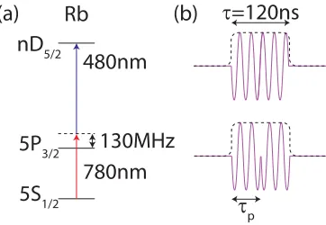
3.2 Experimental setup. (a) Rydberg atom excitation scheme. (b) RF signal sent to the acousto-optic modulator used to control the upper transition laser pulse for the case without phase inversion (top) and with phase inversion at time𝜏𝑝 (bottom). . 42
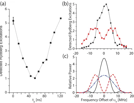
Excitation spectra without phase inversion (black squares) and with phase inversion at𝜏𝑝= 60 ns (red circles). c) Power spectra of three different square pulses. Black
line: 𝜏 = 120 ns and constant phase. Red dashed line: 𝜏 = 120 ns and phase flip at 𝜏𝑝=𝜏/2. Blue dash-dotted line: 𝜏 = 60 ns square pulse without phase flip and
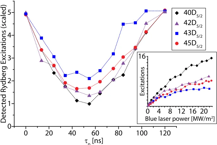
with twice the intensity of the other two pulse types. . . 45 3.4 Number of Rydberg atoms detected as a function of 𝜏𝑝 for the states 40D5/2
(black diamonds), 42D5/2(green triangles), 43D5/2 (red circles), and 45D5/2(blue squares). For ease of comparison, all curves are scaled to a value of five at 𝜏𝑝 = 0
and 120 ns. The inset shows the number of Rydberg atoms detected as a function of upper transition laser power for the same set of states. The degree of saturation reflects the strength of atom-atom interactions. . . 47 3.5 Echo visibilities (squares, left axis) and calibration factors (circles, right axis) for
each𝑛-state examined. The points in this graph follow a very similar trend because of the correlation between saturation of Rydberg atom excitation and loss of echo visibility. . . 48 3.6 Excitation spectra for the states 42D5/2, 43D5/2, and 45D5/2. The black squares
show the case where the excitation amplitude is constant throughout the pulse, and the red circles show the results when𝜏𝑝=𝜏/2. The number of detected excitations
is scaled to give a maximum excitation number of five. . . 50 3.7 Ratio of⟨𝑑−lm𝑝⟩to [2𝑟b]−𝑝 for𝑝= 1, 3, and 6 and𝑟b= 5𝜇m. . . 52 4.1 Effect of atom size on ponderomotive level shifts of Rydberg atoms in an optical
lattice. a) The level shifts are averages over the free electron ponderomotive po-tential (dotted curve; maximum height 𝜅𝑒−) weighted by the Rydberg electron’s
density distribution. Hence, the lattice potentials of large Rydberg atoms tend to be shallower than those of small ones (sold curves; maximum height 𝛼𝑛𝜅𝑒−,
with state-dependent reduction factors 0 < 𝛼𝑛 < 1). b) Calculated frequency
shift, (𝛼𝑛+1−𝛼𝑛)𝜅𝑒−, of the Rb𝑛S→(𝑛+1)S transition at a lattice maximum as a
function of principal quantum number,𝑛. . . 59 4.2 a) Diagram of laser beams used for Rydberg excitation and for creating the optical
lattice. b) Offset foci of the 780 nm and 1064 nm beams. . . 62 4.3 Laser excitation spectra of the 50S Rydberg level for the dipole trap and optical
lattice, obtained by scanning the upper transition laser. The dashed vertical line represents the approximate maximum lattice-induced shift. Clearly, this estimate of the maximum shift is accurate only to within a few MHz, as it is difficult to tell exactly when the signal drops to zero. . . 63 4.4 Lattice spectra as a function of the retroreflection lens position. Count rate is
plotted on a log scale to show extra detail in low-count regions. The black arrows point to regions where the atoms experience a local maximum in the light shift (see text). . . 64 4.5 Dipole trap and lattice spectra as a function of 1064 nm laser power. Count rate
is plotted on a log scale to show extra detail in low-count regions. . . 65
create the optical lattice, because this adds a running wave component to the field and results in an offset energy shift for both the ground and excited states. This shift does not depend on the Rydberg state. . . 66 4.7 Rydberg electron trap depth as a fraction of the free electron trap depth versus the
principal quantum number for nS1/2states of Rb. . . 67 4.8 Dependency of the Rydberg trap depth on𝜂. . . 71 4.9 Microwave spectra of the 50S→51S transition outside of the lattice and for three
different lattice-induced shifts. The thick green line shows the results of a numerical simulation (see text). (For clarity, spectra are staggered vertically.) . . . 72 4.10 Microwave spectra of the 62S→63S and 68S→71S transitions. (For clarity, spectra
are staggered vertically.) . . . 75 5.1 Phase-space diagram for motion of atoms in a ponderomotive optical lattice. The
different shaded regions correspond to the trajectory classes A, B, and C seen in Figure 5.2. . . 79 5.2 Experimental microwave spectra (dots and thin lines) of the 50S→51S transition
outside of the lattice and for a Rydberg lattice modulation depth of𝑉0= 10 MHz. The shaded curve shows the result of a simulation. The coloring of the shaded curve corresponds to the coloring of the different regions of Figure 5.1. . . 80 5.3 Calculated 𝑆0.01-subset of Rydberg atom trajectories in a ponderomotive optical
lattice for the same parameters as in Figure 5.2 and for the indicated values of the microwave detuning (-430 kHz, -80 kHz, and 40 kHz from top to bottom). The histograms on the right show the corresponding probability distributions along the 𝑧-coordinate. . . 84 5.4 Contour plot of microwave spectra of the 50S → 51S transition as a function of
microwave detuning and lattice phase shift after excitation. . . 88 5.5 Rydberg atom trajectories for the indicated amounts of lattice shift after excitation.
The right side of each graph contains a histogram of z-positions in the lattice. The sine waves overlaid on the right show the locations of the lattice maxima and minima relative to the trajectories and the histograms. . . 91 5.6 Three-dimensional intensity profiles for an optical lattice with equal beam sizes (a)
and for two beams with a spot size ratio of ten to one (b). . . 92 5.7 Two example trajectories of atoms in the potential shown in Figure 5.6b. Both
atoms are three-dimensionally trapped, as a result of the attractive radial force that follows from the potential shown in Figure 6b. The inner turning point results from a centrifugal potential. . . 93 6.1 Adiabatic potentials in wavenumbers, 𝑊, for an optical lattice with 𝑉0=2 GHz,
𝑛 = 30 and𝑚𝑗 = 2.5. These potentials exhibit distinct regions of approximately
linear and quadratic behavior, explained in the text. . . 100
6.3 Adiabatic potentials for an optical lattice with 𝑉0=2 GHz,𝑛= 65 and 𝑚𝑗 = 2.5
(panel (a)) and 𝑚𝑗 = 32.5 (panel (b)). For 𝑚𝑗 = 2.5, because of the extent of
the Rydberg atom wave-function, there are no longer clear distinctions between different regions of the lattice, as the wave-function of the Rydberg atom averages over many parts of the potential. For𝑚𝑗 = 32.5, the number of states is reduced
and the linear- and quadratic-like regions reemerge (see text). . . 102
6.4 Splitting between adjacent adiabatic potential lines at the inflection point of the lattice for𝑚𝑗=2.5 (a) and𝑚𝑗=𝑛-2.5 (b). The splitting values for𝑚𝑗 =𝑛−2.5 are multiplied by a factor of two (see text). The solid line shows the splitting predicted by the effective electric field model. . . 104
6.5 Wave-function amplitude squared for an 𝑛 = 30 atom at 𝑧0 = 0 for three dif-ferent states, and the corresponding set of adiabatic potentials. Wave-functions and potentials are calculated without fine structure or quantum defects. (a) The lowest-energy adiabatic potential is a state that is purely vibrational and thus ex-tends along the axis of the lattice. (b) The wave-functions for higher energies compared to that shown in (a) gain more excitation transverse to the axis of the lattice. (c) The highest-energy adiabatic potential corresponds to a state that is purely rotational, extending in the plane transverse to the lattice axis. (d) Adia-batic potentials near𝑧0= 0. The black dots identify the energies and locations for which the wave-functions are calculated. . . 110
6.6 A closer look at the adiabatic potential for a 𝑉0 = 2 GHz lattice with𝑛= 30 and 𝑚𝑗 = 2.5 reveals three classes of states. Class I consists of vibrational states with a positive dipole moment, class II consists of vibrational states with a negative dipole moment, and class III consists of rotational states. . . 112
7.1 Initial telescope used to create a slightly divergent beam. . . 115
7.2 Birefringent calcite crystal used to separate the incident beam into two polarization components. . . 116
7.3 Recollimation of two spatially separated beams. . . 117
7.4 Focus of the two beams into the vacuum chamber. . . 117
7.5 Complete optical setup for dual excitation beams. . . 118
7.6 Intensity profile of two spatially separate excitation beams overlayed with a dipole trap profile. Fit parameters represent a fit to each individual peak. . . 119
7.7 Excitation scheme for Raman optical lattice. . . 120
7.8 Dressed state picture for Raman optical lattice. . . 121
B.1 Coupling between the 5S1/2 state and the 5P3/2 state due to a static electric field. 131 B.2 Energy levels near the 5S-5P transition in Rubidium (left). Dressed state energy levels with a 1064 nm field (right). . . 132
B.4 Origin of the three different peaks in the dipole trap spectra. . . 136 B.5 Dipole trap spectra as the 5S-5P laser is scanned in frequency. . . 137 B.6 Spectrum of atoms in and out of the dipole trap with a 1 GHz detuning on the
intermediate transition. . . 138 C.1 Normal (index) surfaces for the ordinary and extraordinary rays in a negative (𝑛𝑒<
𝑛0) uniaxial crystal. . . 140 D.1 Plot of𝑦= sin𝑥and𝑦=𝑥/√(2). . . 143
Appendix
A. Atomic U nits . . . 126
A.1 Interaction Energy Vint . . . 127
A.2 Ionization electric field . . . 128
B. Scalar, Tensor, and Dynamic Polarizabilities of Atoms . . . 129
B.1 Scalar and Tensor Polarizabilities . . . 129
B.2 Dynamic Polarizability . . . 131
B.3 Dynamic Polarizabilities: On Resonant Dipole Trap Spectra . . . 132
C. Phase Matching in a Frequency-Doubled Laser . . . 139
D. Calculating the Fourier transform limit of an optical pulse . . . 142
I examine interactions between ensembles of cold Rydberg atoms, and between Rydberg atoms and an intense, optical standing wave. Because of their strong elec-trostatic interactions, Rydberg atoms are prime candidates for quantum information and quantum computation. To this end, I study excitation dynamics in many-body Rydberg systems using a rotary echo technique similar to the echo sequences used in nuclear magnetic resonance schemes. In this method, a phase reversal of a narrow-band excitation field is applied at a variable time during the excitation pulse. The visibility of the resulting echo signal reveals the degree of coherence of the excitation process. Rotary echoes are measured for several 𝑛D5/2 Rydberg levels of
rubid-ium with principal quantum numbers near 𝑛 = 43, where the strength of electro-static Rydberg-atom interactions is sharply modulated by a F¨orster resonance. The Rydberg-atom interactions diminish the echo visibility, in agreement with theoretical work. The equivalence of echo signals with spectroscopic data is also examined.
Applications of Rydberg atoms based on controlled interactions require a trap-ping device that holds the atoms at well-defined positions several microns apart.
Rydberg atoms in ponderomotive optical lattices present a unique platform to meet this requirement, as well as to study properties and interactions of these highly ex-cited atoms. Because the Rydberg electron is so loosely bound, the ponderomotive interaction for a Rydberg electron is very similar to a free electron. Ponderomotive lattices tailored to trap Rydberg atoms will allow new experiments in quantum
powerful technique to probe the motion and to verify trapping of Rydberg atoms in ponderomotive lattices. The potentials for non-degenerate, low angular momentum states, are used to obtain ensembles of Rydberg-atom trajectories in the lattice, and to simulate the spectra of microwave transitions of Rydberg atoms moving through the lattice. Additionally, adiabatic potentials are calculated for Rydberg atoms in one-dimensional ponderomotive lattices for a variety of atomic states and lattice pa-rameters. The lattice induced mixing of nearly-degenerate, high-angular-momentum states is explained in terms of effective electric and magnetic fields.
Introduction
Rydberg atoms have attracted significant interest in the scientific community over the past several decades due to their unique, exaggerated properties. These atoms are characterized by their large sizes, strong electro-static interactions, and polarizabilities that scale with principal quantum number to the seventh power, resulting in extreme sensitivity to external fields. The name “Rydberg atom” is in honor of the Swedish physicist Johannes Rydberg, who introduced the Rydberg formula and the Rydberg constant as an empirical way to determine the energy of the spectral lines in hydrogen. The formula also applies to other species of atoms, and is an excellent approximation for highly excited Rydberg atoms. These atoms have an outer electron that is excited into a very high energy state, i.e. a state of high principal quantum number 𝑛. When this occurs, the atom behaves essentially like a very large hydrogen atom, with a loosely bound outer electron at a high radial separation from the positive ion core. Rydberg atoms are often used in experiments pertaining to quantum information [1, 2], but are also used in other contexts. For example, Rydberg-Rydberg molecules can be created from multipole forces that bond two Rydberg atoms at large internuclear distances [3–6]. Ref. [3] suggests a number of interesting possibilities for the use of such molecules, such as studying collective
excitation, and the creation of superposition states between free and bound atoms. Rydberg atoms can also spontaneously evolve into a plasma [7] and vice versa. Some of the first experiments in plasma formation were conducted by the Rolston group at the National Institute of Standards and Technology in Gaithergsburg, MD [8– 10]. An ultracold plasma formed via ionization of cold Rydberg atoms is a unique state of matter that can have temperatures four orders of magnitude smaller than conventional cold plasmas. Such ultracold plasmas have applications to antihydrogen formation [11] and even quantum information [2]. Because the strong interactions of Rydberg atoms persist over long ranges (10’s to 100’s of microns), these atoms are also often studied in the context of many-body physics [12–15].
1.1 Rydberg atom properties
Because of the Rydberg atom’s similarity to a hydrogen atom, the Bohr model works well as a first approximation for many of the Rydberg atom’s properties. For example, balancing the centripetal acceleration of the Rydberg electron and Coulombic force from the nucleus gives us
𝑚𝑒𝑣2
𝑟 =
𝑒2
4𝜋𝜖0𝑟2 (1.1)
where 𝑚𝑒 and 𝑣 are the electron’s mass and speed, respectively. Quantizing
angular momentum in units ofℏ (𝑚𝑒𝑣𝑟=𝑛ℏ) immediately leads to the relationship
𝑟= ℏ2
(𝑒2/4𝜋𝜖0)𝑚𝑒𝑛2 =𝑎0𝑛2 (1.2)
where 𝑎0 is the familiar Bohr radius. This is an important result which tells us
frequency, 𝜔=𝑣/𝑟, of the Rydberg electron:
𝜔2 = 𝑒2/4𝜋𝜖0
𝑚𝑒𝑟3 . (1.3)
From Equations 1.2 and 1.3, we see that the Kepler frequency scales as𝑛−3, which
will be important for later sections of this thesis concerning optical lattices. A number of other scaling parameters can also be derived from the classical description of the atom and are summarized in Table 1.1. Two particularly relevant scalings include the electric field at which the Rydberg atom ionizes, which will be important in state selective detection of Rydberg atoms, and the dipole-dipole interaction (proportional to the dipole moment squared), which is the basis for many of the studies in this thesis.
To determine the ionization electric field for a Rydberg atom, I begin with the combined Coulomb-Stark potential given by
𝑉 =−1𝑟 +𝐸𝑧 (1.4)
where 𝐸 is an electric field applied along the z direction and 𝑟 is the radius of the Rydberg electron orbit. This equation is written in atomic units which are summarized in Appendix A.2. The saddle point of this potential, found by setting the derivative equal to zero, is located at𝑧 =−𝐸−1/2 where the potential is −2√𝐸.
This means that an electric field of𝐸 =𝑊2/4, where𝑊 is the binding energy of the
𝐸 = 161𝑛∗4 (1.5)
where 𝑛∗ is the effective principal quantum number, 𝑛−𝛿
𝑙 [16]. This derivation
works very well to estimate the ionization electric field, but ignores the fact that as the ionization electric field is increased, the atoms undergo a Stark shift and may mix with nearby energy levels. The atom may traverse the Stark map adiabatically (staying in its original energy level) or diabatically (hopping to other nearby levels) depending on both the speed of the electric field ramp and the size of the avoided crossings. Diabatic traversal of the Stark map will broaden the ionization signature and result in ionization electric fields ranging from 1
4𝑛∗4 to 9𝑛1∗4 [16].
The dipole-dipole interaction is the interaction energy of a dipole in the electric field of another dipole. The dipole moment of an atom is given by ⃗𝜇 = 𝑒⋅r and scales like 𝑛2. The electric field of a dipole at a location R is the result of the field
from the nucleus which scales as 1/𝑅2, and the field of the electron which scales as
−1/(𝑅+𝑟)2. The sum of these fields for large distances R can be approximated as
𝑟/𝑅3, or 𝑛2/𝑅3. This results in a dipole-dipole interaction energy of 𝑉
dd ∼ 𝑛4/𝑅3.
It is important to note that in the context of the Rydberg atom experiments dis-cussed here, the atoms do not have permanent dipole moments, and therefore the dipole-dipole interaction is a result of transition dipole moments to other states. Additionally, I have left out the angular dependence of the derivation of the dipole-dipole interaction energy. The complete form of the interaction energy is given by
𝑉dd = ⃗𝜇1⋅⃗𝜇2−3 (𝑅⃗𝜇13⋅𝑛ˆ) (⃗𝜇2⋅ˆ𝑛) (1.6)
where ⃗𝜇1 and ⃗𝜇2 are the transition dipole moments of the two atoms involved
Binding energy 𝑛−2 Energy between adjacent states 𝑛−3
Orbital radius 𝑛2
Dipole moment 𝑛2
Polarizability 𝑛7
[image:23.612.232.408.69.156.2]Radiative lifetime 𝑛3 Rabi frequency for excitation 𝑛−3/2 Table 1.1: Scaling laws for Rydberg atoms.
Table 1.1 contains many of the Rydberg atom scalings that will be important for this thesis.
1.2 Rydberg atoms for quantum information
The application of Rydberg atoms to quantum computing is perhaps the most significant driving force behind the study of these exotic atoms. Here I will briefly explain recent developments in the field and how Rydberg atoms can be used to gen-erate quantum gates. There are several excellent references in which the reader can find more detailed information [1, 2, 17] as well as the Quantum Information Science and Technology Roadmap website, operated by Los Alamos National Security, LLC, at http://qist.lanl.gov/.
get smaller and smaller. However, we can instead take advantage of these effects by using the principle of superposition.
A classical computer uses bits of information stored as 1s or 0s, while a quantum computer is capable of storing any superposition of these two states. While at the end of the computation the superposition state is destroyed and the result must be read out simply as one of the two states, the advantage of the quantum nature of the system lies in the computation itself. One can show that a quantum computer can be simulated by a classical computer, but it is impossible to perform this simulation efficiently. This means that quantum computers offer an essential speed advantage over classical computers. In fact, this speed advantage is so immense that many researchers believe that no conceivable amount of progress in classical computation would ever be able to close the gap between the classical and quantum computation domains [17, 18].
quantum systems that were too complicated to be simulated on a classical computer could in fact be simulated on a quantum computer, which would have huge scientific and technological implications. The bottom line is that although we still do not know all of the benefits that quantum computing has to offer, it is certain that it will become the future of computing.
For successful quantum computation, one must create a quantum bit, or qubit, that can exist in one of two states labeled ∣0⟩and ∣1⟩. In 2000, David DiVincenzo of IBM laid out some requirements for a successful quantum computer. These include scalability, the ability to initialize the qubits, gates fast enough to avoid the effects of decoherence, a universal gate set (meaning that any arbitrary operation can be completed), and the ability to read out an answer. What kinds of qubit systems show promise for the creation of a quantum computer? There are several different avenues that are all simultaneously being explored1. Popular systems include trapped
ions [19], neutral atoms [20], semiconductor quantum dots [21], cavity QED [22], and NMRbased systems [23].
Ions are one of the most promising candidates because they are easily trapped and have strong interactions via the Coulomb force. The strong interactions mean that gate operations can be completed quickly. However, just like the ions interact strongly with each other, they are also capable of interacting strongly with their environment, which leads to decoherence. Neutral atoms provide the opposite sit-uation. They interact more weakly with their environment than ions, but at the same time gate times are longer because they also interact weakly with other atoms. Alternatively, Rydberg atoms provide the best of both of these worlds.
Rydberg atoms, though neutral, interact very strongly with each other. This
1The website mentioned earlier, http://qist.lanl.gov/, contains roadmaps for all of the current quantum
R
1
0
|
|
|
ω
|
00
|
01
|
10
|
11
|
00
|
01
|
10
|
11
Figure 1.1: Rydberg atom fast phase gate first proposed by Jaksch et al. in 2000.
allows quantum gates to be completed quickly, as in the case of trapped ions. An additional advantage that ions do not have is the fact that the interaction can be tuned and even switched off for a desired amount of time. This can be done either by Stark shifting the Rydberg state with an electric field, or by de-exciting the atom from the Rydberg state. Once the interaction is turned off, the coherence can be preserved because as mentioned above, the neutral atom does not interact strongly with its environment. Lastly, because Rydberg atoms are significantly larger than their ground-state atom counterparts, they are more easily accessible (i.e. they can be individually addressed with laser beams) for quantum computing applications.
The first Rydberg atom quantum gate was proposed by Jaksch et al. in 2000 [1]. This proposal was for a two-atom fast phase gate taking advantage of the dipole-dipole interaction that prevents more than one Rydberg atom from being excited at one time (see Section 1.3). This gate involves hyperfine ground state levels, labeled
∣0⟩and∣1⟩, and one Rydberg state. A laser couples∣0⟩to the Rydberg level, while∣1⟩
applied to atom A. The idea is that for every case except for ∣11⟩ (where there is no coupling of the atoms to the Rydberg state at all), the excitation blockade prevents the second atom being excited. This results in a phase shift for every state except
∣11⟩. The truth table for such a gate is shown on the left-hand side of Figure 1.1. Later, Lukin et al. showed that this same idea could be applied to a mesoscopic ensemble of atoms via entanglement [2].
Since then, a number of exciting advances have been made in the field of quantum information processing with Rydberg atoms. Particularly, in 2009, Phillipe Grang-ier’s research group from Laboratoire Charles Fabry and Pierre Pillet’s research group from Laboratoire Aim´e Cotton demonstrated collective excitation of two atoms each held in a separate dipole trap [24]. This experiment was a major step forward in quantum-information science as well as in many-body physics in general because it was the first time anyone had successfully demonstrated the excitation blockade with individual atoms. They also observed an enhancement of single-atom excitation proving the coherent behavior of their system. In early 2010, Grangier’s group gen-erated an entangled state with the same system of spatially separated dipole traps with a fidelity of 0.75 [25]. At the same time, a research group at the University of Wisconsin demonstrated a controlled-NOT gate with a fidelity of 0.58 [26].
1.3 Rydberg atoms and the excitation blockade
0R 1R 2R
[image:28.612.250.392.68.237.2]h
ω
Figure 1.2: Rydberg excitation ladder.
shorthand notation for the number of Rydberg excitations that are coherently shared among all atoms in the excitation region of our experiment until a measurement is made that projects that excitation onto a single atom. The ket ∣0R⟩ represents a system where all atoms are in the ground state, and the ket ∣1R⟩ is sum over all possible configurations where a single atom is in the Rydberg state. It is somewhat inaccurate to label the second excited state with the ket∣2R⟩because this is a doubly excited state and its energy will depend on the distance between the excited atoms. However, it will suffice for the treatment in this thesis.
Here, I have labeled the energy difference between the states ∣0R⟩ and ∣1R⟩ as
ℏ𝜔. If the atoms were non-interacting, then one would expect that the ∣1R⟩ → ∣2R⟩
transition energy would also beℏ𝜔. However, because of the afore mentioned strong interactions, the ∣2R⟩ state is shifted in energy. The size and direction depends on the Rydberg state [27], but if the magnitude of the shift is greater than the linewidth of the optical source used for excitation, then the ∣2R⟩ state is out of resonance, and all excitation above ∣1R⟩ is blockaded.
have non-zero transition-dipole-moments to the states 𝐵 = ∣𝑛′, 𝑙′, 𝑗′, 𝑚′
𝑗⟩ and 𝐶 =
∣𝑛′′, 𝑙′′, 𝑗′′, 𝑚′′
𝑗⟩. The infinite-separation energy defect is defined as Δ =𝑊𝐵+𝑊𝐶 −
2𝑊𝐴. It is then found that the second order shift, Δ𝑊(2), is given by
Δ𝑊(2) =− ∑ 𝑛′,𝑙′,𝑗′,𝑚′
𝑗, 𝑛′′,𝑙′′,𝑗′′,𝑚′′
𝑗
∣⟨𝑛′′, 𝑙′′, 𝑗′′, 𝑚′′
𝑗∣ ⊗ ⟨𝑛′, 𝑙′, 𝑗′, 𝑚′𝑗∣𝑉dd∣𝑛, 𝑙, 𝑗, 𝑚𝑗⟩ ⊗ ∣𝑛, 𝑙, 𝑗, 𝑚𝑗⟩∣2
Δ
(1.7) where𝑉ddwas defined in Equation 1.6. Equation 1.7 is sufficient to find the energy
shift of an arbitrary state ∣𝑛, 𝑙, 𝑗, 𝑚𝑗⟩ as long as the Rydberg atom does not possess
a permanent dipole moment. Low angular momentum states of rubidium Rydberg atoms do not have a permanent dipole moment unless an external field is applied at a sufficient strength [28].
In general, the sum in Equation 1.7 will have contributions from many two particle states. If none of the interaction channels (2𝐴↔𝐵+𝐶) are resonant (i.e. Δ≫𝑉dd),
then the system is considered to be in the off-resonant, van der Waals regime. In this case, the interaction induced energy shift scales as𝑉2
dd/Δ or𝑛11/𝑅6, as is evident from
Equation 1.7. However, there are cases in which a resonant interaction channel (Δ≪
𝑉dd) exists. In this case, the non-degenerate perturbation treatment in Equation 1.7
is not accurate. Here, the system is in the on-resonant, dipole-dipole regime, and the interaction induced energy level shift is calculated via degenerate perturbation theory. One then finds that the energy left shift scales as 𝑉dd or 𝑛4/𝑅3. These
subject in numerous contexts [14, 29–31].
1.4 Properties of Rubidium
All of the experiments in this thesis use 85Rb. Alkali-metal atoms (lithium,
sodium, potassium, rubidium, cesium, and francium) are popular for Rydberg atom experiments as well as for atomic physics experiments in general. For one, their ex-citation frequency from the ground to the first excited state is in the visible part of the electromagnetic spectrum. Laser light at these frequencies is increasingly easy to generate, and indeed, alkali-metal atoms were the first to be cooled and trapped. It is also an easy task to generate an atomic beam because of the large vapor pressure of these atoms. All alkali-metal atoms have a closed electronic core with a single valence electron. This means that the state of the electron is completely determined by its orbital and spin angular momenta, 𝑙, and 𝑠, since the closed electronic core does not contribute.
There are three important temperature scales to consider when cooling and trap-ping 85Rb [32]. The first of these is referred to as the capture limit. When resonant
light is shined on an atom moving at a high speed, the Doppler shift may cause the light to be far enough out of resonance that the atom cannot absorb the photons’ energy. For 85Rb, this velocity is equal to
𝑣𝑐 = 𝛾𝑘 = 2𝜋×6 MHz× (
2𝜋 𝜆
)−1
= 4.7 m/s (1.8)
where𝛾 is the linewidth of the transition and𝜆is the frequency. This corresponds to a temperature of
𝑇𝑐 = 𝑀𝑣
2 𝑐
where 𝑀 is the mass of Rubidium and 𝑘𝐵 is the Boltzmann constant.
The next temperature scale is the Doppler limit, which is the energy corresponding to the natural linewidth of a transition. The Doppler limit arises because of the randomness of spontaneous emission (necessary for laser cooling), which causes the atom to move on a random walk and therefore competes with cooling. The Doppler temperature gives us a limit of how effective Doppler cooling can be for a particular species of atom, although sub-Doppler cooling often allows much lower temperature almost by accident [33]. The Doppler temperature and velocity are given by
𝑇𝐷 = 2ℏ𝑘𝛾
𝐵 = 144 𝜇K (1.10)
𝑣𝐷 =
(
𝑘𝐵𝑇𝐷
𝑀
)1/2
= 11.8 cm/s. (1.11)
Lastly, the recoil limit, as the name suggests, corresponds to the energy gained or lost through the absorption or emission of one photon by the atom. For Rb,
𝑣𝑟 = ℏ𝑀𝑘 = 0.6 cm/s (1.12)
𝑇𝑟 = 𝑀𝑣
2 𝑟
𝑘𝐵 = 0.37𝜇K (1.13)
There are two rather inventive ways of optically cooling below the recoil limit, including Raman cooling [34] and Velocity Selective Coherent Population Trapping (VSCPT) [35]. These methods allow one to reach a temperature in the 100’s of nanoKelvin range. Below this, for example to achieve BEC, non-optical techniques such as evaporative cooling are necessary [36]. In this thesis, I focus on atoms
1.5 Thesis framework
This thesis is organized as follows: In Chapter 2, I begin with a summary of the experimental apparatus used to conduct the experiments described in the re-mainder of the thesis. Two primary setups were used, referenced as the “Blockade Experiment” and the “CryoMOT”.
Chapter 3 discusses a rotary echo technique I used to demonstrate excitation coherence in a system of Rydberg atoms as a means to overcome the effects of density inhomogeneity. Maintaining the coherence of the system is important in many applications, but most notably in quantum computation where information must be preserved during the course of each gate operation. My experimental effort was initially inspired by a paper written by Francis Robicheaux in 2008 [37]. There, it was suggested that rotary echo schemes could be used to quantify coherence in a mesoscopic ensemble of atoms. Previously, coherence was measured by observing Rabi oscillations of cold, trapped atoms between the ground and excited Rydberg state. However, the number of atoms in a system had to be limited to one or two in order to measure such coherence, since interactions between Rydberg atoms quickly caused dephasing in the Rabi oscillations of neighboring atoms [38]. Also in 2008, Tilman Pfau’s research group published their results on applying the rotary echo technique to a 3.8𝜇K sample of rubidium atoms with a density of 5.2×1013cm−3[39].
This was a remarkable achievement because it allowed the measurement of excitation coherence in a large ensemble of atoms - a system much easier to produce than a single isolated atom.
of atom-atom interactions on echo visibility. I was able to measure a rotary echo in a 1 mK sample of atoms with a density of 2.5×1011 cm−3. This experiment is the
first in which an echo signal was observed for a system of atoms with a temperature as high as 1 mK and is more applicable to today’s research in quantum computation with Rydberg atoms than the 3.8 𝜇K temperatures used in [39]. I show how echo visibility depends strongly on the strength of Rydberg-Rydberg interactions, and explain the results in terms of the theory described in Ref. [39]. I also show that the interpretation given in this paper is inaccurate for certain cases in which an increased interaction strength between Rydberg atoms appears to induce a reduction in the observed echo signal. Even more importantly, this echo technique can be used in the future to measure coherence as a function of a wide variety of parameters, including atom temperature, density, interaction strength, and interaction time. In this way, systems designed for quantum computation can be easily analyzed in terms of their coherence properties.
The fundamental parts of the atom trap and imaging system used to measure rotary echoes were designed and built by Tara Cubel-Liebisch and Aaron Reinhard. After their graduation, I designed the system of electronics used to generate the rotary echo sequence and wrote all of the software used to record and analyze the echo signals. I also designed and engineered a system of crossed-beam excitation to narrow my excitation region from several millimeters to about ten microns. Additionally, this system is capable of dual excitation regions produced by diffraction in a non-linear crystal, a feature that will be useful in future endeavors.
studying coherence, I examine the ponderomotive optical lattice as a novel method of Rydberg atom storage that will allow atoms to be individually addressed for qubit initialization and readout. And because the lattice can be precisely tailored using the lattice laser beams, it also allows for scalability of the system. The experiment described in Chapter 4 constitutes the first evidence of a ponderomotive optical lattice for Rydberg atoms. The theoretical existence of such a lattice had been suggested in Refs. [40] and [41], but never observed experimentally. Not only does this trap localize the atoms in space, but it also confines the atoms in micron-sized, spatially separated potential wells such that the atoms to be individually addressed via focused laser beams. This work was featured on the front page of the National Science Foundation website at www.nsf.gov as well as the front page of the University of Michigan website at www.umich.edu.
The experimental apparatus used in this experiment was built by Alisa Walz-Flannigan and Brenton Knuffman. After their graduation, I added the optics to generate a focused optical lattice at the center of the excitation region, and was the first to experimentally observe and characterize the effects of the lattice by using optical and microwave spectroscopy (detailed in depth in Chapter 4).
In Chapter 5 I calculate the trajectories of Rydberg atoms in optical lattices in order to better understand the experimental results shown in Chapter 4. The results of the simulations prove the effectiveness of microwave spectroscopy as a tool to characterize the efficiency of the optical lattice as a trapping device. The simulations used in this chapter were written by Prof. Georg Raithel. I performed the calculations and analyzed the resulting spectra and trajectories.
in classical mechanics. Deeper lattice potentials than those achieved in experiments described in Chapter 4 will be necessary to observe these effects experimentally. The simulations used here were also written by Georg Raithel. Analysis of my results using the simulations was done by Georg and myself.
Experimental Apparatus
I performed the experiments described in this thesis using two primary exper-imental designs. I will refer to these two designs as the “Blockade Experiment” and the “CryoMOT”. In this chapter, I will discuss the basic principles common to all experiments, and then describe the important differences between the Blockade Experiment and the CryoMOT.
2.1 Laser cooling and magneto-optical trapping of atomic vapors
Room temperature atomic vapors are made up of atoms with velocities of ap-proximately 300 m/s. However, since we are concerned with studying atom-atom interactions, we desire a system where thermal contributions can be neglected. This is achieved prior to Rydberg-atom excitation via laser cooling of an ensemble of ground-state atoms. The technique of cooling atoms using radiation pressure is an integral part of many atomic physics experiments today, and has opened entirely new domains of physics since its advent. Prior to the development of laser cooling, stud-ies of atomic samples were all performed with fast-moving atoms, which can make measurements very difficult. Spectral resolution was limited because of the limited observation time, as well as the displacement and broadening of spectral lines due to the Doppler shift and relativistic time dilation. One of the biggest motivations for
developing laser cooling was the limitation on atomic clock performance. Laser cool-ing also helped lead to many new phenomena such as Bose-Einstein condensation [42] and quantum logic gates [43] The technique of laser cooling was first developed using ions trapped with electric fields, and led to the award of the 1997 Nobel prize in physics to Steven Chu, Claude Cohen-Tannoudji and William Phillips.
85
Rb
F=2
F=3
F’=1
F’=2
F’=3
F’=4
5P
3/25S
3/2
C
y
cling
Repumper
[image:37.612.209.440.227.583.2]3 GHz 29 MHz 61 MHz 120 MHz
Figure 2.1: Hyperfine levels of the 5S1/2and 5P3/2 levels in85Rb.
direction, and, after many thousands of scattering events, there will be a signifi-cant cooling effect along the direction of the laser beam. Cooling in all directions is accomplished by applying three pairs of counter-propagating beams in orthogonal directions.
Laser cooling is accomplished using a “cycling” transition, meaning that the atom will absorb and re-emit in a closed sequence of atomic states. Figure 2.1 shows the hyperfine levels of 5S1/2 and 5P3/2 levels in 85Rb. For simplicity, the 𝑚𝐹 sub-levels
are not shown, but we apply 𝜎+ polarized light such that the atoms are always in
the extreme 𝑚𝐹 states. The cycling transition is from 5S1/2, ∣𝐹 = 3⟩ → 5P3/2,
∣𝐹′ = 4⟩. However, because the ∣𝐹′ = 4⟩state is separated from the∣𝐹′ = 3⟩by only
120 MHz, about one out of every 1600 photons scattered will off-resonantly excite into the ∣𝐹′ = 3⟩ state. From here the atom can decay into the ∣𝐹 = 2⟩ manifold,
which is 3 GHz detuned from the cycling transition. Therefore, a “repumper” laser must be used to transfer the atom back to the cycling transition. This laser is tuned to the ∣𝐹 = 2⟩ → ∣𝐹′ = 3⟩ transition.
The limits of this technique arise from the fact that the atoms will undergo a random walk as they spontaneously emit absorbed radiation. Laser cooling is ca-pable of reaching temperatures near the Doppler limit: 144 𝜇K, or 11.8 cm/s for Rubidium. Thus, we can reduce the velocity of the atoms from the speed of sound to approximately the speed of a mosquito. For more information, C.J. Foot’s Atomic Physics provides an excellent overview of the details of this technique.
of radiation pressure, but are not constrained to remain within of the laser beam path. Therefore, laser cooling alone cannot be used to trap atoms. The addition of a quadrupole magnetic field centered about the trapping region provides a position-dependent restoring force. This kind of setup is referred to as a magneto-optical trap or a MOT, and offers an extremely robust method of cooling and confining atoms.
I I
z
[image:39.612.226.422.204.433.2]ρ
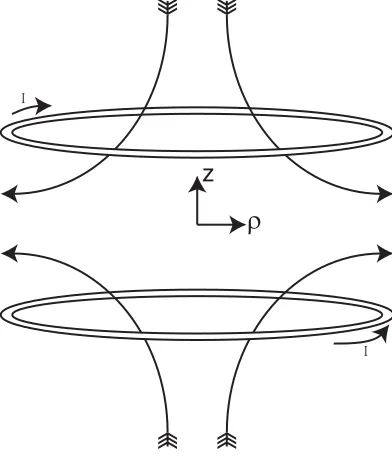
Figure 2.2: The field coils and magnetic field lines of a magneto-optical trap.
Figure 2.2 shows how the magnetic field of a MOT is constructed. Two coils in the anti-Helmholtz configuration create the necessary quadrupole field. The force on an atom in a magnetic field is given by
−
→𝐹 =−→∇(−→𝜇 ⋅−→𝐵) (2.1)
where −→𝜇 is the magnetic moment of the atom. The magnetic field −→𝐵 is given by
𝐴(𝜌2+ 4𝑧2)1/2 (2.2)
we have 𝐵 =𝐴𝑟√4 cos2𝜙+ sin2𝜙: a linear field gradient when𝜙 is constant. This
gradient produces the energy level structure for the Zeeman levels of the trapped atom shown in Figure 2.3. This example is for a simple 𝐽𝑔 = 0 → 𝐽𝑒 = 1 system,
but easily extends into more complicated atom structures where 𝐽𝑔 →𝐽𝑒 =𝐽𝑔+ 1.
z Energy
M
g = 0
Me = +1
Me = -1 Me = 0
Figure 2.3: Zeeman splitting of the first excited state due to the linear magnetic field gradient.
We can take advantage of this Zeeman splitting by choosing the correct polariza-tion for our cooling and trapping light. If the beam has frequency 𝜔𝑙 with 𝜎+ light
incident from the left, and𝜎− light is incident from the right, the excitation scheme
will look like that shown in Figure 2.4:
z Energy
Mg = 0 Me = +1
M
e = -1
M
e = 0
σ+ σ
-Z'
ω
δ+
δ
[image:40.612.185.473.182.349.2]Consider an atom at position 𝑧′. This atom is much closer to resonance with the
light if it is in the 𝑀𝑒=−1 Zeeman sub-level than if it is in the𝑀𝑒 = +1 level. If it
is in the𝑀𝑒 =−1 level, it can only scatter light from the𝜎− beam (and vice versa),
and therefore it will be preferentially scattered to the left. The reverse situation occurs when 𝑧′ is located on the other side of the magnetic field zero.
It is of practical importance to remember the polarizations used for the MOT beams depend on the chosen frame of reference. In the figures in this section, the polarizations are with respect to the atoms, not to the beam axis. With respect to the beam axis, both beams along a single axis have the same polarization (either LCP or RCPwith respect to the direction of travel). The strong axis of the magnetic field (vertical in Figure 2.2) will have the opposite polarization from the other two axes. An easy way to guarantee the polarizations are the same along each axis is to retroreflect the beams with a 𝜆/4 waveplate and a mirror.
In the Blockade Experiment, a vapor cell MOT of 85Rb generates a trap with a
density of about 1010 atoms/cm3 and an atom number of ∼ 106. The diameter of
the MOT is about half a millimeter. We achieve a larger, more dense atom sample by using a two-MOT setup where the vapor cell MOT serves as a primary trap to load a secondary trap located inside an ultra-high-vacuum chamber. In this way, atoms can be collected and cooled in the high-pressure vapor cell MOT, and then transferred into the low-pressure chamber where collision-induced atom loss rates are suppressed.
The transfer from the primary MOT to the secondary MOT is accomplished using a resonant beam with 𝜎+ polarization that drives the 5𝑆
1/2, ∣𝐹 = 3, 𝑚F⟩ → 5𝑃3/2,
∣𝐹′ = 4, 𝑚′
F = 4⟩cycling transition of85Rb. This creates a stream of atoms that move
type of system is often referred to as a Low Velocity Intense Source, or, LVIS [44]. Using the LVIS, we obtain MOTs with a density of approximately 5×10¹⁰atoms/cm3
and an atom number of 5×10⁶.
2.2 Imaging
2.2.1 Calculating atomic sample parameters
Atom numbers and densities are determined using a shadow imaging technique where resonant light is directed onto the atomic sample and “shadow” cast by the atoms is measured with a CCD camera. We define𝐼0(𝑥, 𝑦) to be the intensity profile
of the incident laser beam and 𝐼(𝑥, 𝑦) to be the profile of the beam after passing through the trap. A brief calculation can show that the area density of the atoms is given by
𝑁𝐴(𝑥, 𝑦) = 2Γ𝐼ℎ𝜈
sat ln
𝐼(𝑥, 𝑦)
𝐼0(𝑥, 𝑦)
where Γ is the natural linewidth of the transition, ℎ𝜈 is the change in energy due to a single photon of the probe light, and 𝐼sat is the saturation intensity. Note that
this requires that 𝐼 ≪𝐼𝑟𝑚𝑠𝑎𝑡 such that there are no line splittings and the linewidth
of the transition is not broadened.
The total atom number, 𝑁, can be calculated by assuming the distribution
𝑁𝐴(𝑥, 𝑦) =𝑁𝐴(0,0)𝑒𝑥𝑝(−𝑥
2+𝑦2
𝜎2 ) (2.3)
𝑁𝑉(𝑥, 𝑦, 𝑧) = 𝑁𝑉(0,0,0)𝑒𝑥𝑝(−𝑥
2+𝑦2+𝑧2
𝜎2 ) (2.4)
which also gives the useful result:
𝑁𝑉(0,0,0) = 𝑁𝜎𝐴(0√𝜋,0) (2.5)
2.2.2 Direct versus 4F imaging
The imaging system used to collect the light for the shadow image can greatly
affect the resolution that is obtained. If the shadow image is shone directly onto a
CCD camera, the resolution is given by
1.22𝜆𝑓
𝐷atoms (2.6)
where 𝜆 is the wavelength of the light, 𝑓 is the distance from the atoms to the
camera, and 𝐷atoms is the diameter of the atom cloud. For reasonable experimental
conditions, the amount of blurring seen for a 1 mm MOT cloud is on the order of 100
microns. However, for a smaller atomic sample, such as the dipole trap discussed in
Section 2.3, the atoms would be completely obscured by diffraction. In this case, we
use a system known as 4F imaging, illustrated in Figure 2.5.
f 2f f
Figure 2.5: 4F imaging system for improved resolution of small atomic samples.
1.22𝜆𝑓
𝐷lens (2.7)
where now we have the diameter of the lenses in the denominator instead of the diameter of the atom cloud. This makes it possible for imaging of atom clouds with diameters of 10’s of microns, provided a camera with small enough pixel size is used. A pixelfly high performance digital 12 bit CCD camera with a pixel size of 6.7 𝜇m produces the images shown in Figure 2.6. Both of these images are formed using 4F imaging. While it would be possible to directly image the MOT, the dipole trap with a 15 𝜇m diameter would be not be resolvable. Additionally, a further advantage of a 4F imaging system is that high frequency noise can be reduced by putting a filter on-axis between the two lenses.
~300μm
15μm
a)
b)
Figure 2.6: Images obtained with a 4F imaging system. a) Magneto-optical trap, density 5× 10¹⁰ atoms/cm3, atom number 5×10⁶. b) Optical dipole trap, density 5×10¹¹ atoms/cm3, atom number 3×10⁴.
2.3 Optical dipole traps
by creating an optical dipole trap after atoms are trapped in the MOT. Dipole traps are based on the light shift (AC Stark shift) that atoms experience in an intense laser field. Depending on the detuning of the dipole trap laser, a potential will be created for ground state atoms that attracts them to either the laser intensity maximum (red detuning) or minimum (blue detuning).
Dipole traps need to balance the dipole force with the radiation scattering force in order to trap effectively. For the derivation below, we assume a two-level atom but the equations extend easily to multi-level atoms. The two-level assumption is reasonable in this case because in 85Rb, the transition from the 5S
1/2 ground state
to the intermediate 5P manifold dominates the contribution to the light shift and scattering rate. The interaction potential of the induced dipole moment of a two-level atom in an oscillating driving field is given by
𝑈dip(−→𝑟) = 3𝜋𝑐
2
2𝜔3 0
Γ
Δ𝐼(−→𝑟 ) (2.8)
where Γ is the linewidth of the transition between the two levels, 𝜔0 is the laser
frequency, Δ is the laser detuning from resonance, and 𝐼(−→𝑟 ) is the intensity profile of the laser. The scattering rate is given by
Γsc(−→𝑟 ) = 3𝜋𝑐 2
2ℏ𝜔3 0
(
Γ Δ
)2
𝐼(−→𝑟). (2.9)
Equation 2.9 is obtained after applying the rotating wave approximation and assuming that 𝜔/𝜔0 ∼ 1 (𝜔 is the transition frequency between the two levels of
the atom). From these equations, we see that the potential scales as 𝐼/Δ and the scattering rate scales as 𝐼/Δ2. Because of this, optical dipole traps usually use large
Because the light shift of the atomic states is proportional to the intensity of the laser beam, by focusing the laser beam through the MOT, a potential well can be created that traps the atoms. The spatial intensity of a focused Gaussian beam with power 𝑃 propagating along the z-axis is given by
𝐼FB(𝑟, 𝑧) = 𝜋𝑤22𝑃(𝑧)exp
(
−2𝑤2𝑟(2𝑧)
)
(2.10)
with
𝜔(𝑧) = 𝜔0(1 + (𝑧/𝑧𝑟)2)1/2 (2.11)
𝑧𝑟 =𝜋𝑤20/𝜆 (2.12)
where 𝜔(𝑧) is beam waist and 𝑧𝑟 is the Raleigh length.
The optical potential can be determined from Equation 2.8:
𝑈dip(−→𝑟 ) = 3𝜋𝑐
2
2𝜔3 0
Γ Δ
2𝑃
𝜋𝑤2(𝑧)exp
(
−2𝑤2𝑟(2𝑧)
)
. (2.13)
The depth of the trap is given by ˆ𝑈 =∣𝑈(𝑟= 0, 𝑧 = 0)∣. We see that the potential in the radial direction is much steeper than in the axial direction, since 𝑧𝑟 is a factor
of 𝜋𝑤0/𝜆 larger than𝑤0. Our dipole trap is formed with a 5W, 1064 nm laser beam
fall out of the excitation region. This generates the cigar shaped trap shown in Figure 2.6.
2.4 Rydberg atom excitation
I excite 85Rb Rydberg atoms out of the dipole trap or the MOT using the
two-photon transition 5S1/2 →5P3/2 →nS,nD. The wavelengths for the lower and upper
transitions are 780 nm and 480 nm, respectively. Transitions to states that are not dipole-coupled (nP or nF, for example) can be accomplished as well by applying an electric field across the excitation region. Direction excitation from the 5S state into the Rydberg state can also be done using an ultraviolet laser at 297 nm [45]. A single-photon transition has the advantage that only one laser is required. However, UV light is difficult to generate at the required intensity and the matrix elements coupling the 5S1/2 state into the Rydberg state are much smaller than those for the
two-photon transition. For these reasons, only the two-photon transition scheme is used here.
2.4.1 External cavity diode lasers
To generate a single-mode beam, the laser waveguide must be on the order of the optical wavelength, such that only one mode is supported and a diffraction limited beam is formed.
The wavelength of the laser is determined by the semiconductor material and the modes of the optical cavity. One can tune the diode over a range of a few nanometers by adjusting the current density and the temperature of the diode. Adjusting the injection current will change the refractive index of the active area, which in turn changes the length of the cavity. Temperature influences both the path length and the gain curve of the semiconductor.
A diffraction grating placed after the collimation lens of the diode is also used to adjust the lasing wavelength. This arrangement is known as the Littrow configura-tion. The first order reflection off the grating is directed back into the diode, while the zeroth order is used as the laser output. There is a trade-off between stabilizing the laser with as much reflected power as possible, and still achieving the desired output power. In some cases, up to 50% of the power is reflected back into the diode.
2.4.2 Frequency doubled lasers
Ideally the conversion efficiency can approach 30 percent. The wavelength of the light can be adjusted via grating and current feedback (as discussed in Section 2.4.1 by about ±20 nm. After exciting the shutter of this laser, the 480 nm laser beam is coupled into an optical fiber and directed toward the atoms trapped in the vacuum chamber.
Part of the fundamental 960 nm beam is also coupled out of the system before it enters the doubling cavity. This beam has about 2-3 mW of power. It is used both to measure the wavelength of the laser, and is sent into a pressure-tuned, temperature stabilized Fabry-Perot cavity to stabilize the laser frequency.
2.4.3 Frequency stabilization of diode lasers 2.4.3.1 Saturated absorption spectroscopy
Our home-built, 780 nm diode lasers are stabilized to a Rb reference cell using saturated absorption spectroscopy. The Doppler broadened line shape of a gas of atoms is given by the Boltzmann distribution 𝑒−𝑚𝑣2
𝑧/(2𝑘𝐵𝑇). A laser beam interacts
with atoms that have a given velocity class,
𝑣𝑧 =
(
𝜈−𝜈1
𝜈1
)
𝑐 (2.14)
where 𝜈 is the laser’s frequency and 𝜈1 is the resonance frequency. The number
of atoms absorbing is a Gaussian of the form,
𝑒−𝑚𝑐2(𝜈−𝜈1)2/(2𝑘𝐵𝑇 𝜈12) (2.15)
The full width at half-maximum is therefore
Δ𝜈1/2 =
√
8𝑘𝐵ln 2𝜈𝑐1(𝑇/𝑀)1/2 (2.16)
Probe Ref
Pump
PD Rb Cell
Figure 2.7: Beam configuration for saturated absorption spectroscopy.
When the pump and probe beams are not on resonance with an atomic transition, they interact with different velocity classes since they are counterpropagating (Figure 2.8). Only when they are on resonance will they interact with the same atoms (velocity class 𝑣𝑧 = 0). This causes reduced absorption for the probe beam because
the pump beam depletes the ground state atom population. This is observed by a narrow depression within the Doppler-broadened line. When the reference beam is subtracted such that the two Doppler signals cancel, this depression is the only feature that appears.
probe pump
ngs
v
z
0
Figure 2.8: Pump and probe beams interacting with different velocity classes.
When two transitions share a common ground state and differ in frequency by less than the Doppler width, cross-over peaks occur. From Figure 2.9, it is clear that at some frequency, the same atoms will be resonant with 𝜈1 by the probe and 𝜈2 by
ν2 probe ν2 pump
ngs
v
z
ν1 probe
ν1 pump
0
Figure 2.9: The origin of cross-over peaks.
𝜈1 =𝜈cross− 𝑣𝑐𝑧1𝜈cross (2.17)
𝜈2 =𝜈cross+ 𝑣𝑐𝑧1𝜈cross (2.18)
Solving for the cross-over frequency results in
𝜈cross= 𝜈1+2 𝜈2 (2.19)
The peaks generated using this method of saturated absorption spectroscopy have a width of a few MHz and act as a suitable signal for locking the 780 nm lasers. Feed-back to stabilize the laser frequency is provided by a lab-built PID servo connected to the current of the laser for fast feedback and the grating of the laser for slow feedback.
2.4.3.2 480 nm lasers
2.4.4 Excitation region and detection of Rydberg atoms
MCP
Phosphor
Field
Ionization
Electrodes
Dipole
[image:52.612.228.417.104.254.2]Trap
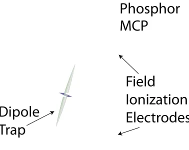
Figure 2.10: Qualitative view of beam geometry in the Rydberg excitation region and the detection electronics used for determining the number and state distribution of excited Rydberg atoms.
Figure 2.10 shows the 780 nm and 480 nm excitation beam geometry for the
Blockade Experiment. The cigar shaped dipole trap is shown in the center (dipole
trap beam not shown). The two beams are focused at the excitation region and
propagate in orthogonal directions. Since the beam geometry changes slightly for
the individual experiments presented in this thesis, further details on the geometries
will be elucidated in each chapter.
As