Link to Leeds Beckett Repository record: http://eprints.leedsbeckett.ac.uk/3341/
Document Version: Article
The aim of the Leeds Beckett Repository is to provide open access to our research, as required by funder policies and permitted by publishers and copyright law.
The Leeds Beckett repository holds a wide range of publications, each of which has been checked for copyright and the relevant embargo period has been applied by the Research Services team.
We operate on a standard take-down policy. If you are the author or publisher of an output and you would like it removed from the repository, please contact us and we will investigate on a case-by-case basis.
For Review Only
H∞ Preview Control of a Class of Uncertain Discrete-Time Systems
Journal: Asian Journal of Control Manuscript ID RR-16-0296.R2
Wiley - Manuscript type: Regular issue: Regular paper
Date Submitted by the Author: 04-Oct-2016
Complete List of Authors: Li, Li; University of Science and Technology Beijing, School of Mathematics and Physics
Liao, Fucheng; University of Science and Technology Beijing, School of Mathematics and Physics
Deng, Jia; Leeds Beckett University, Leeds Sustanibility Institute
Keywords: augmented error system, preview control, robust tracking, uncertain system, observer, LMI
Abstract:
This paper investigates the problem of H∞ preview tracking control with robust performance for uncertain discrete-time systems. In order to avoid applying the difference operator to the time-varying matrix, by taking advantage of the difference between the system state variables, input variables, and the corresponding auxiliary variables, instead of the usual difference between system states, an augmented error system including previewed information is constructed, which converts the tracking problem into a regulator problem. A sufficient condition based on the free-weighting matrices technique and the Lyapunov stability theory is derived for the robust asymptotic stability of uncertain systems. Moreover, a state feedback control law with preview action design method is obtained via linear matrix inequality (LMI) approach. Based on these, a state observer for preview control systems is formulated. Previewable reference signals are fully utilized through reformulation of the output equation while designing the state observer. The proposed construction method of augmented error system is applicable to uncertain discrete-time system in which the uncertainties are general. Also an integrator is introduced to ensure the closed-loop system tracking performance with no static error. The numerical results also show the effectiveness of the preview control law for uncertain systems in the paper.
For Review Only
H∞ Preview Control of a Class of Uncertain Discrete-Time Systems
Li Li Fucheng Liao
School of Mathematics and Physics, University of Science and Technology Beijing,
Beijing 100083, China
Jiamei Deng
Leeds Sustanibility Institute, Leeds Beckett University, Leeds, UK LS2 9EN
Abstract: This paper investigates the problem of H∞ preview tracking control with
robust performance for uncertain discrete-time systems. In order to avoid applying the
difference operator to the time-varying matrix, by taking advantage of the difference
between the system state variables, input variables, and the corresponding auxiliary
variables, instead of the usual difference between system states, an augmented error system
including previewed information is constructed, which converts the tracking problem into
a regulator problem. A sufficient condition based on the free-weighting matrices technique
and the Lyapunov stability theory is derived for the robust asymptotic stability of uncertain
systems. Moreover, a state feedback control law with preview action design method is
obtained via linear matrix inequality (LMI) approach. Based on these, a state observer for
preview control systems is formulated. Previewable reference signals are fully utilized
through reformulation of the output equation while designing the state observer. The
proposed construction method of augmented error system is applicable to uncertain
discrete-time system in which the uncertainties are general. Also an integrator is
introduced to ensure the closed-loop system tracking performance with no static error. The
numerical results also show the effectiveness of the preview control law for uncertain
systems in the paper.
Keywords: augmented error system; preview control; robust tracking; uncertain
system; observer; LMI
1 Introduction
For Review Only
The research question of preview control theory is formulated as follows: when the
reference signal or exogenous disturbance is known or can be previewable, how can we
take advantage of the previewed future desired output signal or disturbance signal to
achieve the best control performance of a closed-loop system? Sheridan proposed the
concept of preview control via three models [1]. Subsequently, for discrete-time constant
coefficient linear systems, Katayama et al. constructed an augmented system that is
equivalent to the original system [2], applying the difference in some degree between the
state variables, tracking error variables. And based on optimal control theory, the optimal
preview controller for the original system was obtained. Tomizuka [3] applied the same
approach as that of Katayama et al. to continuous-time systems and derived an augmented
error system similar to that of the discrete-time system. Finally an optimal preview
controller was obtained by the extremum principle. Due to decades of research, preview
control not only has made a major theoretical breakthrough (e.g., preview control theory of
multirate systems, time-varying systems, continuous-time stochastic systems, and so on
[4-7]), but it also has been used successfully in many other areas [8-10].
Up to now, most existing results for preview control theory are based on deterministic
systems. However, in fact, uncertainty and external disturbance have become the essential
parts of the control systems. Therefore, it is necessary to consider the robust stability and
performance of the preview systems. Using H∞ and H2 optimal control theories, various
studies [11-14] have considered the control problems of preview control systems with
external disturbances and given us the preview control design method. The game-theoretic
approach was introduced into the continuous-time systems to propose the preview control
problems and the state feedback and output feedback were both studied [15]. Subsequently,
Cohen and Shaked [16] employed the method in [14] to discuss the robust preview control
problem for discrete-time systems. Cohen and Shaked [17] proposed the robust H∞
preview control problem for norm-bounded uncertain systems based on the results of [15,
16]. Researchers in [18-20] applied the error system method in [21] to polytopic uncertain
systems to consider the preview control laws design method problems.
Combining the discrete lifting technique with an auxiliary approach, an error system
is constructed and the previewable reference signal is added to the state vector of the
augmented error system. Consequently, the tracking control problem is transformed into
For Review Only
the robust H∞ control problem. Based on this approach, the robust preview tracking control
problem will be discussed. Two appropriate auxiliary variables are introduced to construct
the error system. Therefore, this paper can avoid applying the difference operator to the
time-varying matrix while deducting the formal system. Moreover, the problem over a
finite-time interval that has been only discussed in [6, 12] can then be spread to the infinite
time interval case. For the augmented error system, the state feedback controller and the
reduced-order observer are derived, respectively. The gain matrix of the controller with
preview action design can be transformed to solving linear matrix inequalities (LMIs). The
effectiveness of the results is shown by numerical simulations.
Notations. n
R denotes the n-dimensional Euclidean space and n m
R is n m
matrix space, respectively. A0 means that A is positive definite. AB denotes 0
A B . T
A denotes the matrix transposition of A. I denotes the identity matrix,
and the number of rows and columns can be known from the context of the narrative. The
symbol stands for the transposed elements in the symmetric matrix, that is,
T
X Y X Y
Z Y Z
. sym A( ) denotes
T
AA .
In the following, we give the two lemmas that will be used.
Lemma 1 (Schur Complement Lemma [22])
Suppose matrix 11 12
12 22
T
, where
11 and
22 are symmetric matrices and invertible, then the three conditions are equivalent as follows:(i) 0; (ii) 11 0,
1
22 12 11 12 0
T
;
(iii) 22 0,
1
11 12 22 12 0
T
.
Lemma 2 ([23]) For matrices E and G with appropriate dimensions, uncertain
matrices 1, 2,,s that satisfy T i i I
, i1, 2,,s and arbitrary positive
scalars
1, 2,,
s, the following LMI holds:1
T T T T T
E G G E E E G G,
where diag
1, 2,,s
, diag
1I, 2I,,
sI
. 3For Review Only
2 Problem formulation and basic assumptions
Consider the following uncertain discrete-time system:
( 1) [ ] ( ) [ ] ( ) [ ] ( ),
( ) ( ),
x k A A x k B B u k D D w k
y k Cx k
(1)
where x k( )Rn is the state vector, u k( )Rq is the input control vector,
y k
( )
R
q is the output vector, w k( )Rl is the disturbance vector, and w k( )l2, A, B, C and D are constant matrices with appropriate dimensions. A A k x( , , ) ,( , , )
B B k x
and D D k x( , , ) are uncertain matrices which depend on the
time variable k, the state vector x, or some parameter vector
. In order to ensure theexistence of the state observer of system (1), we assume that
C A,
is observable.Other assumptions are as follows:
Assumption 1:
0
A I B
C
is invertible.
Assumption 1 is the standard assumption for the servomechanism design problem
and shows that the nominal system ( , , )A B C has no zeros at
1.The following is the commonly used assumption in preview control theory about the
predictability of the reference signal:
Assumption 2: The MR future values, (r k1), (r k2),
, (
r k
M
R)
as well asthe present and past values of the reference signal are available at each time k. The
future values of the reference signal beyond the kMR are zero, namely
( ) 0, R 1, R 2, R 3,
r k j jM M M (2)
where MR is the preview length of the reference signal.
And
lim ( )
kr k r, (3)
where
r
is a known constant-vector.It should be point out that (2) is the assumption for the reference signal which
exceeds the preview length and (3) implies that the reference signal is an arbitrary
time-varying function, except that it reaches a steady state.
For Review Only
Remark 1: Theoretical research and practical examples have shown that the
previewable signal has great influence on control effect of the closed-loop system only for
a certain time period during which it exceeds the preview length impact is small; therefore,
the reference signal is assumed to be a constant when it exceeds the preview length. In fact,
a regular feedback control system does not consider the known future information of the
previewable signal, or equivalently, MR0.
Assumption 3: There exist real constant matrices with appropriate dimensions
i
E
,Hi, (i1, 2,3) and uncertain matrices
i i( , , )
k x
such that1 1 1
A E H
, B E22H2, D E33H3, (4)
T i i I
. (5)
Remark 2: In Assumption 3, (4) shows that the uncertain matrices of system (1)
satisfy matching conditions; (5) shows that uncertain matrices are norm bounded. It is
easily seen from expressions A, B and
D
that the uncertainties are associatedwith the state vector or some unknown parameter and may be time varying in nature.
Therefore, the uncertainties referred to in this paper are very general.
It should be noted that the assumption about the uncertain terms in [24] is adopted,
rather than the commonly used assumption in [25]. As mentioned in Remark 2, the above
assumption is more general. In designing the preview controller, if the uncertain matrices
depend on
, then the usual difference method can be used to derive the augmentederror system, see references [18-20]. On the other hand, if they are related to k, the
method in [5] is applicable.
The nominal system of system (1) is
( 1) ( ) ( ),
( ) ( ).
x k Ax k Bu k
y k Cx k
(6)
Motivated by [26-28], we use system (6) to construct the following variables
( ) ( ) ( )
x k x k x k , u k( )u k( )u k( ), (7)
where x k( )、u k( ) are appropriate auxiliary variables. Now a method for selecting
them is given to construct an augmented error system. Define
( ) ( ), ( ) ( ).
x x
u u
(8) 3
For Review Only
If the controlled output of the nominal system (6) for system (1) can track the reference
signal, there exist constant vectors x( ) and u( ) satisfying the equation of system
(6). Thus letting k go to infinity on both sides of equation (6), we obtain
( ) ( ) ( ),
( ).
x Ax Bu
r Cx
(9)
That is,
( ) 0
0 ( )
A I B x
C u r
.
From Assumption 1, take
1
( ) 0
( ) 0
x A I B
u C r
.
Thus, x( ) and u( ) are
( ) ( ) ( ),
( ) ( ) ( ),
x u
x x S r
u u S r
(10)
where
1 00
0
x
A I B
S I
C I
,
1
0 0
0
u
A I B
S I
C I
.
The results of (10) are extended and the auxiliary variables are selected in the followings:
( ) ( ),
( ) ( ).
x u
x k S r k
u k S r k
(11)
Remark 3: As described previously, the auxiliary variables x k( ) and u k( ) will
be used to derive the augmented error system, in order to convert the tracking control
problem into a state feedback H∞ control problem of the augmented error system. The
difference method in [2, 5-6, 17-20] will be found to be the equivalent to the choice of
the auxiliary variables in (7) (i.e., ( )u k u k( 1), x k( )x k( 1)). And the difference
method in [26, 29] is the equivalent of u k( ) u( ) , x k( ) x( ) . Since the
uncertainties are time-varying and unknown in this paper, construction of the augmented
error system through the usual difference method in [2, 5-6, 18-21] is impossible. If we
use u k( ) u( ) and x k( ) x( ), the information on the nominal system cannot be
fully used. Therefore, the method in this paper improves the previous methodologies.
For Review Only
3 Construction of the augmented error system
In this section, an augmented error system which contains the error vector, state of
the system, the future information and the integrator vector will be constructed and the
robust H∞ control for the regulating system will be discussed. The state feedback
controller with integral and preview actions achieving the robust tracking performance in
terms of LMIs is obtained.
Define the error signal as
( ) ( ) ( ).
e k y k r k (12) Combining (1), (7) and (11) gives
( 1) [ ] ( ) [ ] ( ) [ ] ( ) [ ] ( )
[ ] ( ) ( 1),
x
u x
x k A A x k B B u k D D w k A A S r k
B B S r k S r k
(13)
and note that
( ) [ ( ) ( )] ( ) ( ) x ( )
y k C x k x k Cx k Cx k CS r k . (14) Consequently,
( 1) [ ] ( ) [ ] ( ) [ ] ( ) [ ] ( ) [ ] ( ) ( 1),
( ) ( ) ( ).
x u x
x
x k A A x k B B u k D D w k A A S r k B B S r k S r k
y k Cx k CS r k
(15)
Furthermore, obviously have
( ) ( ) x ( )
e k Cx k CS I r k . (16) Using (15) and (16), one can obtain that
( 1) [ ] ( ) [ ] ( ) [ ] ( ) [ ] x ( )
e k C A A x k B B u k D D w k A A S r k
[B B S r k] u ( ) r k( 1)
. (17)
Define
( 1)
1
R
M q R
R
r k r k
X k R
r k M
, [( 1) ] [( 1) ]
0 0
0
0 0
0 0 0
R R
M q M q R
I
A R
I
.
It follows from Assumption 2 that the equation can be obtained
For Review Only
( +1)= ( )
R R R
X k A X k . (18)
Combining (15), (17), and (18) gives
ˆ ˆ ˆ ˆ ˆ ˆ
ˆ( 1) [ ] ( ) [ˆ ] ( ) [ ] ( ),
ˆ ˆ ( ) ( ),
x k A A x k B B u k D D w k
e k Cx k
(19)
where
( )
ˆ( ) ( )
( )
R
e k
x k x k
X k
,
0
ˆ 0
0 0
pe px R
CA G
A A G
A
,
0
ˆ 0
0 0 0
pe px
C A G
A A G
, ˆ
0
CB
B B
,
ˆ
0
C B
B B
, ˆ
0
CD
D D
, ˆ
0
C D
D D
, Cˆ
I 0 0
,and
0 0pe x u
G C AS +BS I , Gpx
AS +BSx u Sx 0 0
,
0 0
px x u
G AS BS
, Gpe
C(ASx BSu) 0 0
C Gpx,where ˆA, ˆB, ˆC and ˆD are constant matrices of the augmented error system, and
ˆ
A
, Bˆ and Dˆ are uncertain matrices.
Note that the main characteristic of system (19) contains the future information on
the reference signal because the variable with future information is a part of the state
variables. Furthermore, by introducing the previewable reference signal, instead of the
difference signal, the signal itself is fully used.
Now considering the previous assumption about the uncertainty, the following will
be obtained.
For Review Only
1 1 1 1 1 1 2 2 2
1 1 1 1 1 1 2 2 2
1
1 2
1 1 1
1 2 1 1 1
2 2
0 ( ) 0 0
ˆ 0 0 0
0 0 0 0
0 0 0 ˆ ˆ
ˆ ,
0 0 0 0
0 0
R
R
R
x u
M
x u
M
M
x u
CE H C E H S E H S
A E H E H S E H S
CE CE
H H S
E E E H
H S
(20)
2 2 2 2
2 2 2 2 2 2 2 ˆ2 2
ˆ ˆ ˆ
0 0
CE H CE
B E H E H E H
, (21)
3 3 3 3
3 3 3 3 3 3 3 ˆ3 3
ˆ ˆ ˆ
0 0
CE H CE
D E H E H E H
. (22)
Note that the uncertain matrices still satisfy the matching conditions
ˆ ˆT i i I
, (i1, 2,3), (23)
and Aˆ, Bˆ and Dˆ are norm bounded.
Note that the augmented system (19) does not contain the difference of u k( ). As a
result, the obtained controller of system (19) based on the LMI approach does not include
the integral of error ( )e k .Therefore, an integrator will not appear in the final closed-loop
system, which helps to eliminate the static error. Due to this reason the discrete integrator is
introduced and defined by
( 1) ( ) ( )
v k v k e k , (24)
namely,
1
0
( ) ( ) (0)
k
j
v k e j v
,where v(0) can be assigned as needed. In general, we take (0)v 0.
Define ( ) ˆ( )
( )
x k X k
v k
again, combining (19) and (24), we get 3
For Review Only
( 1) [ ] ( ) [ ] ( ) [ ] ( ),
( ) ( ),
X k F F X k G G u k H H w k
e k UX k
(25)
where
ˆ 0
E
A F
C I
,
ˆ 0
0 0
A
F
,
ˆ
0
B G
,
ˆ
0
B G
,
ˆ
0
D H
,
ˆ
0
D H
,
0 0
E
C I , U Cˆ 0.
It can be seen from (20), (21), and (22) that the uncertain matrices in system (25)
can be expressed as
1 1 1 1
1 1 11 11 11
ˆ ˆ
ˆ ˆ 0 ˆ
ˆ 0
0
0 0
E
E H
F H E H
, (26)
2 2 2 2
2 2 22 22 22
ˆ ˆ
ˆ ˆ ˆ ˆ
0 0
E
E H
G H E H
, (27)
3 3 3 3
3 3 33 33 33
ˆ ˆ
ˆ ˆ ˆ ˆ
0 0
E
E H
H H E H
. (28)
(23) leads to the fact that the uncertain matrices still satisfy
T
ii ii I
, (i1, 2,3). (29) System (25) is the derived augmented error system. Because ( )e k is the part of the
state vector X k( ), if a feedback control is designed to guarantee the asymptotic stability
of the closed-loop system, then the output y(k) of the closed-loop system of system (1)
can track the desired tracking signal r(k) with no static error.
4 Design of a preview controller
Consider the nominal system of system (25) [ ( )u t 0]
( 1) ( ) ( ),
( ) ( ).
X k FX k Hw k
e k UX k
(30)
Theorem 1: For prescribed 0, system (30) is asymptotically stable with prescribed H∞ performance
, that is, e k( ) 2
w k( ) 2 if there exist matrix P0and matrices T1, T2 with appropriate dimensions such that 3
For Review Only
1 1 1 1 2
2
1 2
1 2 2 2 2
0
T T T T T
T T T T
T T
P U U T F F T T H T F T
= H T I H T
T T F T H P T T
. (31)Proof: Construct the positive definite Lyapunov function according to the matrix P
in (31)
( )
( )T ( )V X k X k PX k .
From (30), for any matrices T1 and T2 with appropriate dimensions the following
equation holds:
1 2
2X k T( )T X k( 1)TT X k( 1) FX k( )Hw k( ) 0. (32)
Calculating the difference of V X k
( )
along the trajectory of system (30) andadding (32) to it yields
2
2
1 2
( ) ( ) ( ) ( ) ( 1) ( 1) ( ) ( )
( ) ( ) ( ) ( ) 2 ( ) ( 1) ( 1) ( ) ( )
T T T T
T T T T
V e k e k w k w k X k PX k X k PX k
e k e k w k w k X k T X k T X k FX k Hw K
( )
( ) ( ) ( 1) ( ) .
( 1)
T T T
X k
X k w k X k w k
X k
Since 0, then V e k e k( )T ( )
w k( )Tw k( )0 for any X k( )0. And the initialcondition X(0)0 implies that e k( ) 2
w k( ) 2, w k( )l2[30-32].Remark 4: The introduction of free weighting matrices leads to the freedom of
some parameters in Theorem 1. Therefore, the conservatism of the solutions can be
reduced. In fact, by setting T10, T2 P, this condition of Theorem 1 is transformed into Lemma 6 in [30]. Actually, based on Lemma 6 in [30], the robust H∞ control
problems were considered by references [31-33]. Therefore, the obtained results may
generalize the relevant results in [31-33].
Now, the purpose of the preview control is to design a state feedback controller for
system (25) in the form of
( ) ( )
u k KX k , (33) such that it makes the closed-loop system of system (25) asymptotically stable. We will
give the controller gain matrix in (33) by using the relevant theory and LMI approach.
For Review Only
From (25) and (33), the following will be obtained:
( 1) [ ( ) ] ( ) [ ] ( ),
( ) ( ).
X k F F G G K X k H H w k
e k UX k
(34)
Theorem 2: Given a scalar 0, a adjustable scalar and a adjustable scalar (0, 2)
, if there exist matrices X 0, Y and constant scalars
i 0, (i 1, 2,3)such that the following LMI holds:
2
2
2
11 1
22 2
33 3
( )
( ) ( 2 )
0
0 0
0 0 0
0 0 0 0
0 0 0 0 0
T
X sym FX GY
H I
X FX GY H X
H X I
H Y I
H I
UX I
,
(35)
where 1 11 11 2 22 22 3 33 33
T T T
E E E E E E
, then system (34) is robustly stabilizable via
(33) and the control gain matrix is given by 1 KYX .
Proof:For the closed-loop system, it can be proved that if (35) is established, then
the conditions of Theorem 1 are established: thus, from Theorem 1, Theorem 2 holds.
For the system (34), it follows from Theorem 1 that given a scalar
0, if there exist P0, T1 and T2 with appropriate dimensions satisfying
1 1 1 1 2
2
1 2
1 2 2 2 2
0
T T T T T
T T T T
T T
P U U T T T H H T T
H H T I H H T
T T T H H P T T
, (36)
where F F
G G K
, then the closed-loop system (34) is asymptoticallystable and satisfies e k( ) 2
w k( ) 2. will be used to denote the left matrix of (36) for simplicity in the following (37), and separated the uncertainties from . Then, together with (26)–(28), the following will be obtained:
1 2 3 3 2 1
T T T
, (37)
For Review Only
where
1 1 1 1 2
2
1 2
1 2 2 2 2
T T T T T
T T T T
T T
P U U T F F T T H T F T
H T I H T
T T F T H P T T
,1 11 1 22 1 33 1
2 11 2 22 2 33
0 0 0
T E T E T E
T E T E T E
, 11 2 22 44 , 11 3 22 33 0 0 0 0 0 0 H H K H .
It follows from (29) that 2 2
T
I
. Lemma 2 is presented to be applied to the
latter two items of the left-hand side matrix in (37), and letting
1 2 3 0 0 0 0 0 0 I I I
,1 0, 2 0, 3 0
, we obtain1
1 1 3 3
T T .
Hence, if there exist
1 0,
2 0,
3 0 such that 11 1 3 3 0
T T
, (38)
then 0, thus, the condition of Theorem 1 is satisfied. Now the necessary and sufficient condition for (38) is discussed. According to the Lemma 1, it follows that (38)
is equivalent to
1 1 2 11 22
2
1 2 33
2 2 3
11 1
22 2
33 3
0
0 0 0
0 0 0 0
0
0 0 0 0 0
0 0 0 0 0
0 0 0 0 0
0 0 0 0 0
T T T T T
T T T T T
T H H K H U
H T I H T H
T H
H I
H K I
H I U I
, (39)
where
1 1 1 1 1 11 11 1 2 1 22 22 1 3 1 33 33 1
T T T T T T T T
P T F GK F GK T T E E T T E E T T E E T
,
2 1 2 1 2 11 11 1 2 2 22 22 1 3 2 33 33 1
T T T T T T T
T T F
T E E T
T E E T
T E E T ,
3 2 2 1 2 11 11 2 2 2 22 22 2 3 2 33 33 2
T T T T T T T
P T T
T E E T
T E E T
T E E T .
The parameter adjustment method [34-35] is proposed, setting
For Review Only
1T aP, T2 bP, (40) where a and b are adjustable scalars. Then, by performing congruence
transformations by an invertible symmetric matrix diag T
1 1, ,I T2 1,I
to (39) and
denoting 1
P X, KX Y, 1
a
, 1b
, it arrives at the condition in Theorem 2, orequivalently (35) holds.
It has been proved that when T1 and T2 are given by (40) and the adjustable
scalars are selected properly, if (35) holds, then (39) and thereby (36) hold. Thus
Theorem 2 is proved.
Remark 5: if (35) holds, then (
22 )
X 0. And from the structure of , we obtain 0, thereby (
22 )
X 0, and combining X 0 yields 0 2.When is considered as a decision variable which should be minimized. The following will be obtained.
Theorem 3: Consider the system (25) with (33). If the following optimization
problem:
1 2 3
, , , , , , ,
min
X Y
(41a)s.t.
2
2
11 1
22 2
33 3
( )
( ) ( 2 )
0
0 0
0 0 0
0 0 0 0
0 0 0 0 0
T
X sym FX GY
H I
X FX GY H X
H X I
H Y I
H I
UX I
(41b)
has a solution
0,
i 0, (i1, 2,3), X 0 and Y. Then the system (34) is robustly stabilizable with disturbance attenuation
by (33) and the control gain matrix isgiven by 1
KYX .
Now we discuss the control input of system (1).
For Review Only
When Assumption 1-Assumption 3 are satisfied, the control input (33) of system (25)
is obtained. The gain matrix K will be decomposed into:
e x R(0) R(1) R( R) v
K K K K K K M K . (42)
Based on (33) and (42), the following will be obtained:
1
0 0
( ) ( ) ( ) ( ) ( ) ( ( ) (0)).
R
M k
e x R v
i s
u k K e k K x k K i r k i K e s v
The main theorem of the paper is presented by synthesizing the above theorems.
Theorem 4: Suppose that Assumption 1-Assumption 3 are satisfied. The controller
of system (1) can be taken as
1
0 0
( ) ( ) ( ) ( ) ( ) ( ( ) (0)) ( )
R
M k
e x R v u x x
i s
u k K e k K x k K i r k i K e s v S K S r k
, (43)where 1
KYX , X 0 and Y can be determined by (41), and (42) determines the relationship between Ke,Kx,KR(0), ,K MR( R), Kv and K; Sx and Su are solved
by (10). And under this controller, the closed-loop system of system (1) can achieve good
tracking of the reference signal.
Proof: When Assumption 1–Assumption 3 are satisfied, the augmented error system
(25) can be derived. If the LMI optimization problem determined by (41) in Theorem 3
has a solution ( ,
1 2, 3, , , ,X Y, ), by Theorem 3, one gets1
( ) ( ) ( )
u k YX X k KX k , (44) the gain matrix K in decomposed into:
1(0) (1) ( )
e x R R R R v
K K K K K K M K YX ,
then (44) can be written as
1
0 0
( ) ( ) ( ) ( ) ( ) ( ( ) (0))
R
M k
e x R v
i s
u k K e k K x k K i r k i K e s v
.
By (7) and (11), the following will be derived:
1
0 0
( ) ( ) ( ) ( ) ( ) ( ( ) (0)) ( )
R
M k
e x R v u x x
i s
u k K e k K x k K i r k i K e s v S K S r k
.Therefore, theorem 4 holds.
In light of the above equation, it is clear that the preview controller of system (1)
consists of five parts. The first part is tracking error compensation, the second part is the
For Review Only
state feedback, the third part is reference preview feed-forward compensation, the fourth
part is the integration of the tracking error term, and the last one is the compensation by
the initial and final values.
Remark 6: An augmented plant including previewed information is constructed by
using the error system method in preview control theory and the discrete-time lifting
technique. Then the robust stability for the augmented error system of uncertain system is
analyzed and a preview controller is designed by combining the robust control theory and
LMI approach. Based on the key ideas above, the design method of the robust preview
controller is presented. Our results extend some recent results of references [11-21].
5 Design of state observer
If the state variables in the original system cannot be measured as feedback state
variables, equivalently the partial variables x k( ) of X k( ) in system (25) cannot be
available. A state observer to reconstruct x k( ) can be constructed. Due to this reason,
each part of the vector X k( ) is rearranged and system (25) is rewritten as
( 1) 0 0 [ ] ( ) [ ] [ ]
( 1) 0 0 0 ( ) 0 0
( ) ( ).
( 1) 0 0 ( ) 0 0
( 1) 0 0 ( )
pe pe
R R R
px px
e k G G C A A e k C B B C D D
X k A X k
u k w k
v k I I v k
x k G G A A x k B B D D
(45)
Considering the observation equation of system (1), the predictability of the
reference signal, and the introduction of the integrator, the observation equation of
system (45) can be taken as
ˆ
( ) Z ( )
Z k C X k , (46) where
[( 1) ] [( 1) ]
0 0 0
0 0 0
0 0 0
R R
q q
Z M q M q
q q
I
C I
I
,
( ) ( ) ˆ ( )
( ) ( )
R
e k
X k
X k
v k
x k
.
For Review Only
If the nominal system of system (45) is observable, there exists a reduced-order
observer with the related theory of a discrete-time observer [36, 37]. Therefore, in the
following, the reduced-order observer is constructed by
0 0( 1) 0 ( ) 0 ( ) 0 0 0 0
0 0 0
0 ( ),
0
ˆ( ) ( ) ( ),
pe
px R
CA CB G
W k A L W k B L u k G L A
I I
CA
A L L Z k
x k W k LZ k
(47)
where n q[ (MR 1)q q]
LR is the observer gain matrix that makes the eigenvalues of
0 0
CA
A L
be located in the unit circle.
Note that if we let L
L1 L2 L3
, where 1n q
L R , 2 [ ( 1)]
R
n q M
L R , 3
n q
L R ,
then 0 1
0
CA
A L A L CA
; as a result, we only need place the poles of the n-order
matrix and the observer is designed without using H∞ control.
Remark 7: The designed observer (47) for the augmented error system (45) is a
reduced-order observer, while it is full-order for system (15). As with the literature [38],
the designed reduced-order observer for the augmented error system and the designed full
observer for the original system are totally different. The output equation of system (45)
contains the information of the previewable reference signal through reformulation of the
output equation. Therefore, the previewable reference signal can be fully utilized in the
design process. In addition, in designing the observer, the eigenvalues of A L CA 1 must
be located in the unit circle and L2, L3 can be selected as needed without increasing the
difficulty of the eigenvalue configuration. And in fact, when an observer is designed for
system (15), L is selected to ensure that A LC is a stable matrix.
For Review Only
Based on the above analysis, the condition of existence of an observer (47) for the
nominal system of system (45) is that the nominal system is observable. In the following,
the PBH rank test [2] will be employed to prove the observability of the nominal system
of augmented error system (45). For the sake of notational convenience, we denote the
state matrix of the nominal system of system (45) with .
Lemma 3: (CZ, ) is observable if and only if ( , )C A is observable and A is invertible.
Proof:By the PBH criteria, (CZ, ) is observable if and only if the matrix
Z
sI
C
has column full rank for any complex s.
From the expression of and CZ, it can be seen that
( 1)
0
0 0 0
0 1 0
0 0
0 0 0
0 0 0
0 0 0
R
pe R
px Z
q
M q
q
sI G CA
A sI
I s I
sI
G A sI
C
I I
I
.
sI is nonsingular for any complex s satisfying | | 0s . By elementary
transformation of the matrix, we have
( 1) ( 1)
0 0 0 0 0 0
0 0 0 0 0 0 0 0
0 0 0 0 0 0 0 0
0 0 0 0 0 0
0 0 0 0 0 0
0 0 0 0 0 0
0 0 0 0 0 0
R R
Z
q q
M q M q
q q
CA sC
sI
A sI A sI
C
I I
I I
I I
.
Thus the matrix
Z
sI
C
has full column rank if and only if
A sI
C
is of full column
rank.
For Review Only
When s0, one gets from elementary transformation of matrix
0
( 1) ( 1)
0 0 0 0 0 0 0
0 0 0 0 0 0 0 0
0 0 0 0 0 0 0 0
0 0 0 0 0 0
0 0 0 0 0 0
0 0 0 0 0 0
0 0 0 0 0 0
R R
Z s
q q
M q M q
q q CA sI A A C I I I I I I .
Thus the matrix
0 Z s sI C
is of full column rank if and only if A has full column
rank, that is, A is invertible.
Lemma 3 holds.
6 Numerical example
In system (1), let
1.4 0.5 0.2 0.1 0 0.90 0 0.19 0.24 0.24 0.97 0.02
0.24 0.24 0.02 0.9
A , 0.2 0 0.2 0.03 B
, C
0 1 0 0
,0.2 0 0.3 0.1 D
, 1
0.2 0 0 0
0 0.2 0 0
0 0 0.2 0
0 0 0 0.2
E
, 1
0.02 0 0 0
0 0.02 0 0
0 0 0.02 0
0 0 0 0
H , 1 2 1 3
0 0 0
0 0.5cos(0.3 ) 0 0
0 0 0.4sin(0.5 ) 0
0 0 0 0.1
a k a k a
, 2
0.2 0 0 0
0 0.2 0 0
0 0 0.2 0
0 0 0 0.2
E , 2 0.02 0.01 0 0.01 H , 4 5 2
0 0.1cos(0.3 ) 0
0 0.1cos(0.3 ) 0 0
0 0 0.02 0
0 0 0 0.02
For Review Only
30.2 0 0 0
0 0.2 0 0
0 0 0.2 0
0 0 0 0.2
E
, 3
0.02 0.02 0.01
0.01
H
, 3 0.
Through verifying,
0
A I B
C
is invertible, and
C A,
is detectable and 1,2
and 3 satisfy (5) for all k. Therefore, the system satisfies the basic assumptions.
The exogenous disturbance is taken as
1.5, 15 60,
( ) 0,
k w k
other
. (48)
The reference signal is taken as
2 30,
( )
0, 30.
k r k
k
,
(49)
Simulations for three situations are performed in the following. The preview lengths
of the reference signal are MR 7, MR 2 with no preview (i.e., MR 0). According to Theorem 3, we use the LMI toolbox of MATLAB to solve matrix variables X , Y
and
in LMI (41); the adjustable variables are selected as
10, 0.5, and thenthe gain matrix 1
KYX and
min=0.98126 in (41) are obtained naturally.When MR 2, the following will be obtained:
7.25749 7.79562 30.05994 0.70340 27.47107 53.73314 7.62783 8.18856 7.25749 ,
K
,
and
7.25749
e
K , Kx
7.79562 30.05994 0.70340 27.47107
,
53.73314 7.62783 8.18856
R
K ,
7.25749
v
K .
When MR 7, K will obtained as follows:
1 14e x R v
K K K K K R ,
7.25749
e
K ,
For Review Only
7.79562 30.05994 0.70340 27.47107
x
K ,
53.73314 7.62783 8.18856 8.68922 8.89846 8.69581 8.05784 7.04074 ,
R
K
7.25749
v
K .
When MR 0, K will be:
e x v
K K K K
7.32823 7.84756 31.05525 0.67990 27.75698 7.34080 .
Take the allowed initial states are assumed as x(0)
0 0 0 0
T and v(0)0.In order to reflect the uncertainty, the uncertain parameters ai (i1, 2,3, 4,5), with the
absolute values no more than 0.5, are taken as random numbers. Note that if the selecting
method for the auxiliary variables x k( ) and u k( ) in [39] is adopted, then the initial
conditions should be decided based on different situations. The proposed method can
avoid the limitation on initial conditions.
The output curves of system (1) are depicted in Figure 1 and Figure 2 plots the
tracking error. We can see that the output y k( ) can all track the reference signal
accurately with the preview length of the reference signal MR7, MR2, and no preview, respectively. From figures1- 3, we can find that the preview controller provides
better performance than the controller with no preview compensation. And the preview
action can reduce the tracking error and the input peak, and accelerate the speed of the
output response tracking the reference signal. This is exactly how preview control
achieves its goal.
For Review Only
0 20 40 60 80
0 0.5 1 1.5 2
k
y
(k
),
r(
k
)
r(k) y,M
R=7 y,M
R=2 y,M
R=0
Figure 1. The output response of uncertain system to step signal.
0 20 40 60 80
-2 -1.5 -1 -0.5 0 0.5 1
k
tr
a
c
k
in
g
e
rr
o
r
M R=7 M
R=2 M
[image:24.612.184.431.85.295.2]R=0
Figure 2. The tracking error of uncertain system to step signal.
In addition, from (10),
1.68977 1.00000 5.55781 0.52632
x
S
and Su 0.05858 can be obtained.
Therefore, the steady-state values of the introduced auxiliary variable x k( ) and u k( )
are given by
For Review Only
( ) lim ( ) 0.11716
k
u u k
,
3.37954 2.00000 ( ) lim ( )
11.11562 1.05264
k
x x k
.
The simulations shows that the steady-state values of x k( ) and u k( ) do tend toward
the steady-state values of the nominal system of system (1). And the steady-state values
of system (1) are close to the steady-state values of the nominal system over time. Here,
as an example, Figure 3 shows the curve of the control input changing in time.
0 20 40 60 80
-10 -5 0 5 10
k
u
(k
)
u,M R=7 u,M
R=2 u,M
R=0
Figure 3. The control input of uncertain system to step signal.
Furthermore, according to Figure 1, it is seen that the closed-loop system has
desirable steady-state response characteristics. The output response curve (i.e., Figure 1)
will be further analysized by using the dynamic characteristics in the following.
The rise time: kr 7, kr 9, kr 10; the delay time: kd 29, kd 35, kd 37; the settling time: ks 34, ks 41, ks 44.
Based on the above, the preview actions can make the closed-loop system has better
dynamic characteristics.
(2) The reference signal is the ramp signal
For Review Only
0, 10,
( ) 0.05( 10) 10 50,
2, 50.
k
r k k k
k
(50)
For the reference signal (50), the simulation will be completed for the following
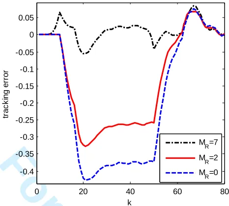
three situations, that is, ①MR7, ②MR 2, ③MR 0. Figure 4 indicates the output of system (1) and the desired tracking signal. Figure 5 shows the tracking error
and Figure 6 plots the control input, respectively. It can be seen from Figure 4 – Figure
6 that the speed of the output response tracking the reference signal is faster and the
adjustment time can be shortened by increasing the preview length of the reference
signal.
0 20 40 60 80
0 0.5 1 1.5 2
k
y
(k
),
r(
k
)
r(k) y,M
R=7 y,M
R=2 y,M
R=0
Figure 4. The output response of uncertain system to ramp signal.
For Review Only
0 20 40 60 80
-0.4 -0.35 -0.3 -0.25 -0.2 -0.15 -0.1 -0.05 0 0.05
k
tr
a
c
k
in
g
e
rr
o
r
M R=7 M
R=2 M
R=0
Figure 5. The tracking error of uncertain system to ramp signal.
0 20 40 60 80
-3 -2 -1 0 1 2 3 4 5
k
u
(k
)
u,M R=7 u,M
R=2 u,M
[image:27.612.181.414.86.296.2]R=0
Figure 6. The control input of uncertain system to ramp signal.
It follows from the simulations of periodic interference signals that the design
control system still has perfect tracking performance and possesses strong disturbance
rejection. And these figures for the results will no longer be presented here due to
considering the length of this paper.
To design the