OPTIMIZATION OF HIGH VOLTAGE POWER SUPPLY FOR INDUSTRIAL MICROWAVE GENERATORS FOR ONE MAGNETRON

(1)

ISSN: 1992-8645 www.jatit.org E-ISSN: 1817-3195

377

PSO-BASED DBSCAN WITH OBSTACLE CONSTRAINTS

1

XIAONING FENG，2ZHUO WANG , 1GUISHENG YIN，1YING WANG

1_{College of Computer Science and Technology, Harbin Engineering University, Harbin 150001, China}

2

National Key Laboratory of Science and Technology on Autonomous Underwater Vehicle, Harbin Engineering University, Harbin 150001, China

ABSTRACT

This paper presents a new PSO-based optimization DBSCAN space clustering algorithm with obstacle constraints. The algorithm introduces obstacle model and simplifies two-dimensional coordinates of the cluster object coding to one-dimensional, then uses the PSO algorithm to obtain the shortest path and minimum obstacle distance. At the last stage, this paper fulfills spatial clustering based on obstacle distance. Theoretical analysis and experimental results show that the algorithm can get high-quality clustering result of space constraints with more reasonable and accurate quality.

Keywords: Space Clustering, Obstacle Constraints ,Particle Swarm Optimization Algorithm, DBSCAN

1. INTRODUCTION

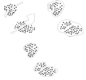
Spatial clustering has been an important data mining field of research. At present, the current clustering methods are dividing methods, hierarchical methods, density-based methods, grid-based methods, genetic algorithm, fuzzy method, rough set, and some clustering algorithms also integrate with a variety of methods. However, these clustering algorithms ignore the existence of many constraints in the real world, and constraints will affect reasonability of clustering results, such as rivers, roads, etc., as shown in Figure 1. Due to the obstacle, the two spatial points close to each other may not belong to the same cluster. In previous work, only a few algorithms in the clustering process considered the impact of the obstacles. However, there are many shortcomings in the aspect of efficiency and quality. Therefore, in order to improve the practicality of clustering, it is not only very important to study the space clustering in constraint environment but also practical in the real world environment.

(A)The Distribution Of Points And Obstacles (B) Clustering Regardless Of Obstacles (C) Clustering

[image:1.612.347.498.329.470.2]

According To Obstacles

Figure 1: Space Clustering With Obstacle Constraints

(2)

378

2. DBSCAN CLUSTERING WITH

OBSTACLE CONSTRAINTS

2.1 Classic DBSCAN Clustering Algorithm

DBSCAN algorithm is a density-based clustering method with high-quality, and applicable to geometry clustering of any shape and size, which can automatically determine the number of clusters, and separate clusters with environmental noise effectively. At first we need to introduce the related concepts of DBSCAN algorithm:

Definition 1: (Core Point) Point has at least

MinPts objects in Epsneighborhood.

Definition 2: (Boundary Point) Point in the core object’s Eps neighborhood, but not meets the

requirements of core object.

Definition 3: (Directly Density-reachable) A point

p

is directly density-reachable from a point

q

if

( )

and

p∈NEps q (1)

( )

NEps q ≥MinPts

︱︱ (2)

Definition 4: (Density-reachable) A point

p

is density-reachable from a point

q

if there is a chain of points P P_{1 2}，，，… P_n P₁=Q，P_n =P such that

1 i

p+ is directly density-reachable from pi.

DBSCAN algorithm efficiency depends on neighbor query and requires inspect each point in data set by checking the neighborhood of each point to find cluster. If a point is a core point, then DBSCAN creates a cluster centered by this point and find directly density-reachable points. The algorithm's time complexity is _{O n}₍ 2₎_{, where}_n_is

the number of points in data sets. If using spatial index, DBSCAN algorithm's time complexity isO n( log )n .

2.2 Improved DBSCAN Clustering Algorithm

With Obstacle Constraints

When traditional DBSCAN algorithm measures the distance of point P and point Q , it uses the Euclidean distance to calculate straight-line distance between two points, which will be unreasonable in the case of obstacles. The existing of obstacles usually makes point P and point Q not visible to each other, that is the connection line of point P and point Q could intersect with obstacles. This paper uses particle swarm algorithm to optimize the obstacles path, and defines the minimum obstacle distance between point P and point Q is the shortest path value of point P and point Q bypass all the obstacles.

Meanwhile, due to the shortcoming of difficulty in discovering clusters with large density difference, this paper uses partition-based DBSCAN clustering method, that is to cluster based on the spatial density distribution of points. Thus, when facing the problem of uneven distribution of data density and cluster density, it will select a smaller value which results in a more dilute Eps cluster divided into multiple similar clusters, and at the same time selecting a larger Eps value will not ignore the differences of larger density.

3. PSO-BASED DBSCAN ALGORITHM

WITH OBSTACLE CONSTRAINTS

3.1 Particle Swarm Optimization Algorithm

PSO (Particle swarm optimization) is an evolutionary computation technique, and firstly introduced by Kennedy and Eberhart in 1995. Similar to genetic algorithm, the study of birds prey behavior is an iteration-based optimization tool. In the PSO algorithm, each optimization problem solution is a bird in the search space, and is abstracted as particles in the N-dimensional space. Particle i in the position of N-dimensional space represents a vector, and the flight speed of each particle is also a vector. Currently, PSO algorithm has been widely used in function optimization, neural network training, fuzzy system control and other applications of genetic algorithms.

PSO initializes to be a group of random particles

(random solutions), and then finds the optimal

solution iteratively. Assuming in d-dimensional

search space the position and velocity of i particle

is i ( _,1 _,2 _, )

i i i d

X = x x x and Vi =(v vi_,1 i_,2vi d_, ) respectively, and during each iteration, particles

update themselves by tracking the two "extreme

value”. One extreme is the best particle solution of

itself, which is the individual extreme

pbest

, and the other extreme is the optimal solution of the

current group, which is the global

minimum

gbest

. When PSO finds out these two optimal values, each particle updates its own pace

and the new location according to the following

formula:

,( 1) ,( ) 1 1[ , ,( )] 2 2[ , ,( )]

i j i j i j i j g j i j

v t+ =wv t +c r p −x t +c r p −x t (3)

, ( 1) , ( ) , ( 1), 1, 2, ,

i j i j i j

(3)

379 In the formula

c

₁and

c

₂are positive learning

factors, generally being equal to 2, at the same time

1

r

and

r

₂are uniformly distributed random numbers between 0 and 1. This paper uses random weight

factor method, setting

w

to a random number with

random distribution, which can overcome the

shortcomings caused by the linear decrease, that is:

* (0,1)

min ( max min) * (0,1)

w N

rand

µ σ

µ µ µ µ

= + 

 = + −

 (5)

In the above formula, N(0,1)is standard random

number with normal distribution, and rand(0,1) is random number between 0 and 1. µmax is the maximum value of random weighted w’s average value. σ is the variance ofw’s random weight, setting to be

max 0.8

µ = ,µmin=0.5andσ =0.2.

3.2Obstacle path optimization based on PSO

Obstacles will inevitably affect the spatial distance between objects, which directly affects the clustering results. When it comes to obstacles, the main solution methods are: view method, grid method, neural networks, artificial potential field, etc. However, these methods all have the defects of search path complexity and inefficiency. This paper combined the theory of mobile robot obstacle avoidance path planning in the dynamic process with particle swarm optimization algorithm to calculate the obstacle distance in the clustering process, which achieved good results and high performance.

Assume S and G are the two objects within many obstacles in the clustering process. The mission for particle swarm optimization is to search a shortest collision-free path between S and G, and the value of this path is the shortest obstacle distance between S and G, the objective function of which is shown as below:

2 2

1 1

2

( ) ( )

p

n

i i i i

i

F x x₋ y y₋

=

∑

− + − (6)

To accelerate the calculation speed, we firstly connect point S and G to be a lineSG, and divide it into n equal portions. Make vertical line of

SGin each divide point, then get

1, 2, , and

L L … Ln.

Secondly starting from point S, we connect each discrete points in all vertical lines, then get a set of discrete obstacle points

(

1 2

)

Obstacle _ path= S P P, , , ..., Pn G, , where

(

1, 2,...,

)

j

P j = n is non-obstacle point and the

line of

j

P and its adjacent points has no obstacle

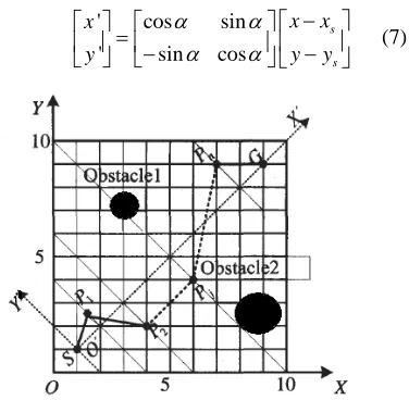
point. At last, we setSG as X-axis, and set the line through S but perpendicular to X-axis as Y-axis, then create a new coordinate system X'OY', which will conduct coordinate transformation to deal with all discrete points ( , )x y in each vertical line.

' cos sin

' sin cos

s

x x

x

y y y

α α

−

 

   

= _ _

  ₋  ₋

[image:3.612.335.523.207.391.2]

      (7)

Figure 2: Coordinate Transformation Model

In the above formula,

α

is the angle value of counterclockwise rotation of original X-axis to line

SG, and

1 1

( ,x y) is starting point S’s coordinate in original coordinate system. In the coordinate system X'OY ', we define S as the

0

P , G as

1 n

P₊ , then simplify _Obstacle_{_}_path encoding to be:

[

1 2

]

_ 0 ' ' n' 0

Obstacle path= y y y (8)

For writing convenience, if no special instructions, we use y instead of y′ . Obstacles distance Obstacle_dist is:

2 2

1 0

_ ( ) ( )

1

n SG

j j

j

L

Obstacle dist y y n +

=

= + −

+

∑

(9)

In the above formula, L_SGis the length of line SG. The search steps of minimum obstacle distance calculation based on PSO are shown as follows:

We select the obstacle distance of starting point S to G as fitness value. The smaller the fitness value, the more optimal solution obtained. Fitness function is shown below:

2 2

1 0

( ) ( ) ( )

1

n

i i

SG

i j j

j

L

F y y y

n +

=

= + −

+

(4)

380 In the above formula, i

j

y presents the

( 1, 2,..., )

j j= n -dimensional position of particle

( 1, 2,..., )

i i= N ; both ends of the

constraintsy₀i =yin+₁=0.

In this paper, we use circles to represent obstacles. In the process of particle swarm initialization and optimization, we not only have to consider the boundary constraints, but also dynamic obstacle avoidance, so we must verify whether the distance between particles location in each dimension and the center of the obstacle circle is greater than the radius of distance circle. The distance between particles location and the center of the obstacledist_{s ob}_{_} is:

2 2

_ ( ) ( )

1

i SG

s ob k k j

L

dist x j y y

n

= − ∗ + −

+ (11)

In the above formula, (x yk, k) denotes the

coordinate of k center of obstacle circle, and

i j

y denotes j j( =1, 2,..., )n -dimensional position of

particles i i( =1, 2,...,N).

In addition, we need to consider whether the line of each particle’s adjacent two-dimensional coordinates intersects with obstacles. The distance between the center of obstacle circle and particle’s adjacent two-dimensional coordinates dist_{ss ob}_{_} is:

_ ₂ ₂

k k

ss ob

Ax By C dist

A B

+ + =

+

(12)

In the above formula, (x yk, k) denotes

k coordinates of the center of obstacle circle,

and A B C, , are determined by the lines of each

particle’s adjacent two-dimensional coordinates as

follows:

1

0 1

( 1) 0

1

i SG

j

i SG

j

L

A j By C

n L

A j By C

n +

 ∗ ∗ + + =

 +



 ∗ ∗ + + + =

 +



(13)

In the above formula, i j

y denotes the

( 1, 2,..., )

j j= n -dimensional position of particle

( 1, 2,..., )

i i= N .

Obstacle path optimization based on PSO steps

are shown as below:

Step 1 Initialize particle dimensionn, particle

numberN . Randomly initialize the position and

velocity of each particle. In initialization process of 0

, i j

y , not only consider boundary constraints, but also consider dynamic obstacle avoidance, which

uses formula (11) and (12) to judge obstacle

avoidance.

Step 2 Calculate the fitness of each particle by

fitness function (10), store particle's current

position and fitness value in pbest, store in the

position of best individual position and fitness

value of each pbest in gbest;

Step 3 Update particle velocity by formula(3).

Step 4 Update particle position by formula (4),

and consider boundary constraints and dynamic

obstacle avoidance.

Step 5 Update weights by formula (5).

Step 6 As for each particle, and compare its

fitness value with its best position pbest, if better,

then set it current best position.

Step 7 Compare all current pbest and gbest

value, and update gbest.

Step 8 Return to step 3, 4 and 5 to iterate until

the algorithm reaches the maximum number of

iterations or meets the accuracy requirements then

when search stops to obtain the shortest path

_ best

Obstacle path and minimum obstacle

distanceObstacle dist_ _best.

3.3 PSODBSCAN Algorithm with Obstacle

Constraints

PSODBSCAN algorithm based on particle swarm optimization with obstacle constraints not only overcomes the shortcoming of classic DBSCAN algorithm, but also can realize dynamic obstacle avoidance which can calculate obstacle distance efficiently. The pseudo code of the PSODBSCAN algorithm is shown as below:

Input: SetObject, Eps, MinPts

Output: Clutering result

Algorithm:

PSODBSCAN(SetObject，Eps，MinPts) {

ObstaclePrint；

For(i=1；i<=SetObject.size；i++) {Object=SetObjeet．get(i)；

IF(Object．ID= =UNCLASSFIED)

{Seed=AcquireNeighbor(SetObject，Object，Eps)

(5)

381

IF(! IsCoreObject(Object，MinPts，Seed)) ChangeID(Object，NOISE)；

ELSE

Cluster(SetObject，Object，Eps，MinPts，Seed)

；

} }

PrintClusteringResult; }

Function ObstaclePrint draws obstacles in the coordinate system, and function AcquireNeighbor (SetObject, Object, Eps) returns all the neighboring objects of Object within Eps, and function IsCoreObject (Object, MinPts, Seed) determines whether Object is a core object, and function Cluster (SetObjeet, Objeet , Eps, Minpts, Seed) returns a set of connected density points. Mealwhile function AcquireNeighbor (SetObject, Object, Eps) needs invoke particle swarm optimization algorithm to determine the minimum obstacle distance, and its pseudo-code is shown as follows:

Input: SetObject, Eps, MinPts

Output: all the neighboring objects of Object

within Eps

Algorithm:

Seed=AcquireNeighbor(SetObject，Object，Eps) {

For(j=1;j<=DensitySet(Object).size;j++) {CheckObject=DensitySet.get(i) ChangeXOY(CheckObject,Object)

Obstacle_distbest= PSO(fitness,N,c1,c2,w,M,D) IF(Obstacle_distbest<=Eps)

Seed.add(CheckObject) }

}

Function DensitySet(Object) returns all the neighboring objects of Object within Eps, and ChangeXOY(CheckObject,Object) transforms coordinates of CheckObject and Object according to formula (5), that is the point S and G denote CheckObject and Object in the coordinate. When

PSO optimization function PSO(fitness,N,c1,c2,w,M,D) initializes and updates

particle position, it needs to verify whether the current position is inside the obstacle or not. Its pseudo-code is shown as follows:

Input: Particle Location，Particle Dimension

Index，Obstacle Circle X coordinate CircleX，

Obstacle Circle Y coordinate CircleY，Obstacle Circle Radius

Output: 0 or 1

Algorithm:

Ob=CheckObstacle(Location,Index,CircleX,Circle Y,Radius)

{

For(k=1;k<=CircleX.size;k++) {Dist1= AcquireDist1(CircleX.get(k),

CircleY.get(k), Radius.get(k),Location,Index); Dist2= AcquireDist2(CircleX.get(k),

CircleY.get(k), Radius.get(k),Location,Index);

IF(Dist1<Radius.get(k)| Dist2<Radius.get(k)) {Ob=1;

break; }

ELSE

Ob=0; } }

Function AcquireDist1(CircleX.get(k),

CircleY.get(k), Radius.get(k), Location,Index)

calculates the distance between the current position

and the center of obstacle circle, that is dists_ob,

and function AcquireDist2(CircleX.get(k),

CircleY.get(k), Radius.get(k),Location,Index)

calculates the distance between the center of

obstacle circle and the value of adjacent two

position line, that is distss_ob. If either Dist1 or

Dist2 exceeds the radius value of obstacle circle,

then we set Ob equal to be 1 and break a loop and

re-allocate position.

4. EXPERIMENTS

Experiment1 Assumed that work space is 100 *

(6)

382 vertical coordinates of all the shortest paths obtained by random weight PSO algorithm, where the 0-dimensional and 20-dimensional both have vertical coordinate value of 50.

Figure 3:The Shortest Obstacle Paths Obtained In Two Experiments

[image:6.612.309.525.108.304.2]

Figure 4: The Relation Curves Of Global Optimum Fitness And Iteration Times In Two Experiments

Table 1. Each Dimension Of The Vertical Coordinates Of Shortest Paths In Two Experiments

NO. 1 2 3 4

Experiment1 52.1932 53.0893 51.4093 50.3336 Experiment2 51.5499 52.4902 53.2507 54.2206

NO. 5 6 7 5

NO. 9 10 11 12

NO. 13 14 15 16

NO. 17 18 19 20

[image:6.612.84.305.396.620.2]

Experiment1 51.5004 51.4360 51.3508 50 Experiment2 44.7523 46.7864 48.6647 50

Table 2 shows two experimental results of view method, traditional PSO algorithm and PSO algorithm with random weights, from which we can see that the optimum values of these three algorithms are obtained in two different environments, with average obstacle distance obtained from two experiments to be average value.

Table 2. Results Comparison Of Three Algorithms

View Method

Traditional PSO Method

PSO Method with Random

Weight

Calcula ted Value

Opti mum Value

Avera ge Value

Opti mum Value

Avera ge Value

Expe rime nt 1

103.928 6

104.2 538

105.1 547

103.9 572

104.4 587

Expe rime nt 2

108.378 5

109.1 532

109.9 726

108.4 472

108.8 359

The experimental results show that PSO algorithm with random weight has better performance than traditional PSO algorithm with higher path searching capability and closer value calculated by view method. In both experiments, the optimum values calculated PSO algorithm have minimum gap, and PSO algorithm with random weight and traditional PSO algorithm are superior to view method in time efficiency. In order to verify whether the experiments have general results, we create many obstacle path problems randomly, and use the same parameters with above three algorithms, similar results obtained.

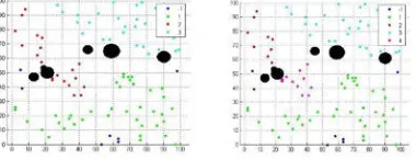
Experiment2 We analyze the clustering of 100

sample objects with no obstacle constraint and many obstacle constraints respectively, and select sample objects including obstacle circles. Figure 5(a) shows the results of PSODBSCAN clustering algorithm. We can see that object points in the same cluster are marked as same color, and object points in the different clusters are marked as different colors, with noise objects marked as dark blue color and ID number equal to -1. Figure 5 (a) shows spatial clustering algorithm result with no obstacle, and Figure 5 (b) shows PSODBSCAN algorithm space clustering results with same sample objects.

[image:6.612.325.515.635.708.2]

(7)

383 The experimental results show that the existence of obstacles affects the continuity of data space, so directly affect the results of space clustering distribution. Contrast Figure 5 (a) and Figure 5 (b), we can see that PSODBSCAN algorithm reflects the impact of spatial obstacles, which divides objects of No.2 category into No.2 and No.4 clusters located at both sides of obstacle circle, and get a more ideal clustering result.

In summary, when at the initial stage particles distribute in the whole solution space, PSODBSCAN has more random character than other algorithm. Meanwhile in each iteration process all the particles share their own “information” and improve their "self-Quality", so that each candidate solution has dual advantages of self-learning and others-learning with fast convergence. At the same time, in the implementation process, as a result of coordinate transformation, PSODBSCAN algorithm reduces computational amount to a large extent, thereby improving execution speed of the algorithm.

5. SUMMARY

Space clustering with obstacle constraints has a strong practical value, and becomes a research focus in field of spatial data mining in recent years. This paper presents a new DBSCAN clustering method based on the PSO optimization, aiming at enriching obstacle path computation method and providing an effective choice for DBSCAN clustering algorithm in obstacle space. The innovation of PSODBSCAN algorithm lies in the reference of mobile robot path planning method, and the simplification of two-dimensional coordinates into one-dimension, then the usage of particle swarm optimization to calculate the minimum obstacle distance between objects, at last the basis of minimum obstacle distance to spatial clustering. Experimental results show that, PSODBSCAN clustering algorithm has not only the advantages of density clustering, but also more reasonability, accuracy in the field of dealing with spatial constraints, which has important theoretical value and significance to achieve accurate clustering in constrained environment.

ACKNOWLEDGEMENTS

This work was sponsored by the national natural science foundation of China under Grant No. 61100006, and the Youth Science Foundation of Heilongjiang Province under Grant No.2007Q0502-00, and the Science Foundation of Heilongjiang Province under Grant No.F201129, and the Youth Science Foundation of Harbin under

Grant No. RC2009QN010039, and the Basic Research Foundation of Harbin Engineering University under Grant No.002060260722, and National Key Laboratory of Science and Technology on Autonomous Underwater Vehicle Foundation under Grant No.2010004, and the Fundamental Research Funds for the Central Universities under Grant No. HEUCF100605.

REFERENCES:

[1] S.R.Feng, W.J.Xiao, “DBSCAN clustering algorithm based on density research and applica-tion”, Computer Engineering and Application, Vol. 43, No. 20, 2007, pp. 216-222.

[2] Ming Song, T.Z.Liu, “Parallel DBSCAN algorithm based on data Partition”, Computer Application Research, Vol. 7, 2004, pp.17-20. [3] Yang.Y, Z.W.Sun, “A method of space

clustering algorithm with obstacle constraints based on density”, Computer Application, Vol. 27, No. 7, 2007, pp. 1688-1691.

[4] Y.Q.Liu, “A clustering algorithm with obstacle constraints based on grid”, Shandong University Journal, Vol. 36, No. 3, 2006, pp.86-90.

[5] Feng Zhang, B.Z.Qiu, “A effective clustering method based on grid”, Computer Engineering and Application, Vol. 43, No. 17, 2007, pp.167-171.

[6] Fan Wen, “Mobile robot obstacle avoidance in unknown environment research”, Harbin Engineering University Journal, Vol. 30, No. 7, 2009, pp.751-756.

[7] Houfei,Qiao, Z.J,Hou, “Based on neutral network intensive learning application in obstacle avoidance”, Tsinghua University Journal, Vol. 48, No. S2, 2008, pp.1748-1755. [8] Lian Duan, Lida Xu, Feng Guo, “A local-density based spatial clustering algorithm with noise”, Information Systems, Vol. 32, 2007, pp. 978-986.

[9] P.Viswanath, Rajwala Pinkesh, “l-DBSCAN:A Fast Hybrid Density Based Clustering Method”, IEEE Proceedings of the 18th International Conference on Pattern Recognition, 36, 2006, pp.34-39.