2016 International Congress on Computation Algorithms in Engineering (ICCAE 2016) ISBN: 978-1-60595-386-1
1 INTRODUCTION
Fire efficiency [1] is the core factor of weapon system, and kill probability is the most important factor in it. The evaluation of a weapon system is the accuracy and efficiency of it. Therefore, firing accuracy is the most necessary factor to be improved, which can not only save a lot of bullets, but also be the core factor to win the whole warfare. Firing accuracy is the meaning of the degree of deviation between aiming point and burst point. Firing error contains the conception of firing accuracy and firing intensity.
Firing table can figure out the firing data to weapon system, but designing a firing table need a lot of shooting experiments and theoretical calculations. There are some methods to design and amend a shooting table before, such as the method of average error which depends on numerous results in shooting tests and the contrast experiment which depends on the same type of bullets [2]. In addition, there are a lot of researches on the influential parameters of firing table and hitting accuracy analysis models designed previously, such as the influential parameters analy-sis[3, 4] hitting probability analysis [5], hitting efficiency function design [6] and so on.
From the previous papers and methods, we know that they are not efficient enough for improving the
accuracy of firing table at a high level. It also needs more work on designing and amending it after using the former methods. Some of them lack of error anal-ysis and error control, while some others lack of the consideration of each parameter that should be in-volved into the simulations. Therefore, it is still a problem that designing a firing table costs a lot of unnecessary consumption of resource.
For improving firing accuracy, reducing the shoot-ing error and theoretical calculations, this paper takes a kind of naval gun for simulation, and gives out a new error anglicising model which is based on DBSCAN (Density-Based Spatial Clustering of Ap-plications with Noise [7–9]. It considers every parame-ter that can influence the hitting accuracy of firing table, and can eliminate noise point in order to opti-mize the firing table in a high accuracy level. Through using the new designed model, we simulated and compared the former methods, and gave out the effi-ciency results from simulations and practical tests of amendment in new designed model.
2 ERROR ANALYSES
2.1 Firing table
Firing table is the data base which is designed for the
A New Method of Firing Table Correction based on DBSCAN
Hao Sun1*, Yong Li1 & Liguo Chen2
1Department of Electronic Information, Northwestern Polytechnical University, Xi’an, Shaanxi, China 2
Systems Engineering Research Institute, Beijing, China
ABSTRACT: Former methods of amending firing table are not efficient for designing a firing table because it wastes time and needs shooting tests and calculation efforts. In order to reduce the unnecessary consumption it costs before and optimise it at a higher level, this paper introduces the concept of error analysis in firing table system and introduces a new optimized algorithm model of firing table. Using the new method model, it gives out the simulated comparison of the results between original firing table data, method of average error and the new method. Within the same meteorological weather, it compares the results with different parameters of the new algorithm model and gives out the performances in different algorithmic situations. Finally, from the simu-lated results and practical tests between different methods, the authors find that the new model not only can re-duce the consumption of resource, but also can be 10% more efficient than the former ones.
Keywords: firing table; new method; DBSCAN
specialized weapon system that can give out the cor-responding relation between firing angle and ballistic data. It is the core part of a weapon system that can be the essential data base to be depended on. The re-search of general firing table [10] provided a certain kind of guidance for designing and amending firing table. Firing table is classified by two parts, namely, basic firing table and amending firing table.
2.1.1 Basic firing table
Basic firing table is the data base that can give out the standard target point which is based on the basic me-teorological weather. Figure 1 shows the firing area and trajectory in standard meteorological weather.
0
V
g
Dq
'
O dq 0
q d g T q
H 0 q h
A
[image:2.516.97.213.212.313.2]P
Figure 1. Standard meteorological weather of the firing area and trajectory.
Basic firing table expression:
{𝜑𝑔= 𝜑𝑔(𝑑𝑞, ℎ𝑞)
𝑡𝑓= 𝑡𝑓(𝑑𝑞, ℎ𝑞) (1)
Or:
{𝑡𝛼 = 𝛼(𝑑𝑞, ℎ𝑞)
𝑓= 𝑡𝑓(𝑑𝑞, ℎ𝑞) (2)
And:
𝛼 = 𝜑𝑔− ԑ𝑞 (3)
In expression (3), 𝛼 is the high angle which is the difference between the angular heights 𝜑𝑔 of the
weapon and the angular heights of the hit point.
2.1.2 Amending firing table
When meteorological weather is not standard, that is to say:
{
∆v0= v0∗− v0
∆τ = τ0− τ0N
∆P = P0− P0N
∆Gb= Gb∗− Gb
ωd= ωd(hq)
ωz= ωz(hq)
ωh= ωh(hq)
az= kzbvdv−2
(4)
When all the parameters above are not 0, we must use amending firing table to amend the firing area calculated by it. In the expression above: 𝑣0∗ and 𝐺𝑏∗
are respectively the actual initial velocity and the weight of the bullet; 𝜏0 and 𝑃0 are respectively the
actual temperature and the air pressure when the ele-vation is 0; 𝑊(ℎ) = (𝑤𝑑(ℎ𝑞), 𝑤𝑧(ℎ𝑞), 𝑤ℎ(ℎ𝑞))𝑇 is
the wind speed based on different height; 𝑎𝑧 is flow
deviation acceleration.
2.2 Barrage deviation model
Definition of barrage deviation [11]: the vector distance
between target path and bullet path.
If target path is 𝐷(𝑡), bullet path is 𝐷𝑑(𝑡).
Ac-cording to the definition above, the norm of barrage
deviation 𝐸 is:
‖E‖ = min‖Dd(t) − D(t)‖ (5) If we define the time when bullet leave the gun
barrel as 𝑡 = 0, there will be the time 𝑡 = 𝑡𝑓 that:
𝑑
𝑑𝑡‖𝐷𝑑(𝑡) − 𝐷(𝑡)‖𝑡=𝑡𝑓 (6)
= 𝑑
𝑑𝑡[𝐷𝑑(𝑡) − 𝐷(𝑡)] 𝑇[𝐷
𝑑(𝑡) − 𝐷(𝑡)]|𝑡=𝑡𝑓
= 2𝑉𝑑∗(𝑡𝑓)𝐸 = 0
Vd∗(t
f) = Ḋd(tf )– Ḋ(tf) = Vd(tf) − V(tf) (7)
𝑉𝑑∗(𝑡
𝑓) is the relative velocity between bullet and
target. Apparently, all the barrage deviation vectors are perpendicular to the relative velocity. Because
after 𝑡 ≥ 0, the relative velocity always exists. So
there must be a relative velocity surface which is per-pendicular to the target centre, and it is called the bal-listic hit surface. Apparently, barrage deviation is the crossing point from bullet path to the ballistic hit
sur-face. When and only when 𝐷𝑑(𝑡) = 𝐷(𝑡), the barrage
deviation will be 𝐸 = 0. It indicates that barrage
de-viation is a two-dimensional vector of the ballistic hit surface.
d
V
*
d
V
V
0
g
x
*
Z
Z
0
f
t
y
y h
0
g
h
g
T
x
Figure 2. Coordinate system of barrage deviation.
The coordinate system of barrage deviation is
𝑦𝑡𝑓
0 is the extended line of 𝑉
𝑑∗; ℎ𝜑𝑔
0 is the axis of
altitude; 𝑥𝛽𝑔
0 is the axis of azimuth; the surface which
consists of 𝑥𝛽𝑔
0 and ℎ
𝜑𝑔
0 is the ballistic hit surface.
We define the two-dimensional vector 𝐄 = 𝑇⃗⃗⃗⃗⃗⃗⃗⃗⃗ 𝑔𝑍∗
which consists of the intersection point between bullet path and ballistic hit surface 𝑍∗ and the origin of
coordinate system 𝑇𝑔. So barrage deviation can be
indicated as follows:
𝐄 = (𝑥𝐸, ℎ𝐸)𝑇 (8)
𝑥𝐸 and ℎ𝐸 are respectively the azimuth deviation
and altitude deviation of the bullet.
3 OPTIMIZED ALGORITHM OF FIRING TABLE
Because weapon system is a sophisticated system in battlefield environment, numerous and independent factors will be the elements which can cause barrage deviation of weapon system. However, the sum of infinite numbers of independent deviations is ap-proximately in normal distribution [12]. We can use Monte Carlo simulation [13] to make all the barrage deviations into a density based figure, and use a new optimized algorithm model which is based on density to analysis barrage deviations in order to amend bar-rage deviations of firing table.
3.1 DBSCAN algorithm
DBSCAN (Density-Based Spatial Clustering of Ap-plications with Noise) can discover dense sample points and noise points among them [14]. So it can rectify and filter the noise points in order to improve the precision of correction. Noise points are the points which are neither border points nor core points.
Definition 1 (border points): Border points are not core points, but they are in the neighbourhood area of a core point.
Definition 2 (neighbourhood area ε): The radius ar-ea of the given object is called neighbourhood arar-ea 𝜀. Definition 3 (core object): If there are points greater than or equal to 𝑀𝑖𝑛𝑃𝑡𝑠 (minimum points) in the neighbourhood area of the given object, it can be called core object.
Definition 4 (directly density-reachable): If there is a given objects set 𝐷, and 𝑝 is in the neighbourhood area 𝜀 of 𝑞. Additionally, 𝑞 is a core object, that we can call object 𝑝 to 𝑞 is directly density-reachable.
Definition 5 (density-reachable): as for a sample set D, if there is an object chain 𝑝1, 𝑝2, … , 𝑝𝑛, 𝑝1=
𝑞, 𝑝𝑛= 𝑝, and 𝑝𝑖∈ 𝐷(1 ≤ 𝑖 ≤ 𝑛), 𝑝𝑖+1 are objects
that directly density-reachable of ε and 𝑀𝑖𝑛𝑃𝑡𝑠, we define the object 𝑝 is density-reachable with 𝜀 and 𝑀𝑖𝑛𝑃𝑡𝑠.
Definition 6 (density-connected): If there is an ob-ject 𝑜 ∈ 𝐷 which can lead 𝑝 and 𝑞 to be
densi-ty-connected with 𝜀 and 𝑀𝑖𝑛𝑃𝑡𝑠, we define it the density-connected from 𝑝 to 𝑞.
Scan all the data set, and find out that a random core point to expand the whole core points is the way SDBSCAN works. The method is to find all the core points which are density-reachable in the neighbour-hood 𝜀 until there is no such point to be expanded. All the other points besides the border are not core points.
3.2 The application of the algorithm model
Because the distribution of barrage deviation is inde-pendent and random, therefore, we can use densi-ty-based method to analyse the barrage deviation in order to rectify deviation in firing table.
The barrage deviation of naval weapon system [15] is 𝑧𝜖𝑅2, and:
z = zx+ zq+ zr+ zb (9)
In formula (11), 𝑧𝑥 is system deviation, 𝑧𝑞 is
strong correlation deviation, 𝑧𝑟 is weak correlation
deviation, and 𝑧𝑏 is uncorrelated deviation.
According to the distribution of barrage deviation in firing processes or use Monte Carlo simulation, we can get the density-based distribution figure that we can use it to analyse barrage deviation in order to sep-arate the noise points and border points.
.
. .
.
.
.
.
.
. .
. .
.
.
a
b
r
r
.
.
[image:3.516.290.424.368.472.2].
Figure 3. Separation process.
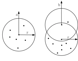
If 𝑀𝑖𝑛𝑃𝑡𝑠 = 4, 𝜀 = 𝑟, the separation process is shown in Figure 3.
The neighbourhood area 𝑟 of point a has 7 points in it, so a is a core point. And there are only 3 points in the neighbourhood area 𝜀 of b. Therefore, b is a border point. Figure 4 is the separation results figure which shows out the results of the separation that it removes all the border points from it.
.
. .
.
.
r.
.
.
[image:3.516.326.387.589.653.2]Apparently, the function of the new algorithm mod-el which is based on DBSCAN is to remove the noise points and reserve the core points which are also the high probability points in firing processes.
The rectified noise of firing table is accurately the amending firing table. Using the results from the new algorithm model can be more efficient in designing and optimizing firing table.
Take the advantages of DBSCAN relevant algo-rithms [16, 17],we can use all the simulated points gen-erated form the shooting tests to optimize firing table.
4 ANALYSIS OF SIMULATION EXAMPLE
For verifying the efficiency feature of the new model, we take a certain type of naval gun as example to do Monte Carlo simulation. Target parameters are as follows: Velocity is 300m/s; fairway crosscut is 500m; altitude is 1000m; horizontal slant distance is 5000m; course direction angle is 210°. Warship parameters are as follows: Velocity is 30 knots; course direction an-gle is 30°. We take the old method of average error used by designing firing table formerly and the new algorithm method which is based on DBSCAN for comparison. The simulated results are as follows.
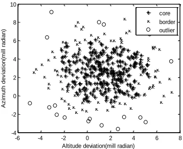
[image:4.516.63.242.497.643.2]4.1 Different parameters in new algorithm model When 𝑀𝑖𝑛𝑃𝑡𝑠 = 10, 𝜀 = 0.4 and simulation times of Monte Carlo are 500, the barrage deviation distri-bution simulated with the parameters shown above is shown in Figure 5. In the figure, core, border and out-lier represent the core points, border points and outout-lier points separately. Obviously, it divides all the points into three different types, namely, core points which are density-reachable, border points which are not core points that can be density-reachable but in the neighbourhood area of a certain core point, outlier points which are noise points that neither core point nor in the neighbourhood area of a certain core point.
Figure 5. Barrage deviation points distribution of new algorithm model.
We can obviously find that the new algorithm mod-el can easily distinguish noise and core points in it which can give us a better correction value.
From the simulated points in Figure 5, we can easi-ly eliminate the noise points in it so that we can use the useful points that really relevant to the barrage deviation system of firing table. Eliminate the noise points and also the border points is the next step for the model. After the eliminating process, we can get the better results from the amending process.
Through using the results, we get from the new al-gorithm model, and we can simulate the system again to see efficiency of the rectified barrage deviation. It costs no resource because we can use previous data we got.
As for the different simulation parameters of the new algorithm model, the simulation results are shown in Table 1 and Table 2. The Monte Carlo time is 500 and the unit of azimuth deviation and altitude devia-tion is mill radian. They show us different results be-tween old method of average error and the method of new algorithm model.
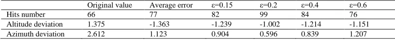
Table 1 shows the results of the comparison be-tween different methods when the constant parameter of the new method is 𝜀 = 0.2 and the variant is 𝑀𝑖𝑛𝑃𝑡𝑠. It shows the different results simulated with different 𝑀𝑖𝑛𝑃𝑡𝑠, they are: 𝑀𝑖𝑛𝑃𝑡𝑠 = 2, 𝑀𝑖𝑛𝑃𝑡𝑠 = 5, 𝑀𝑖𝑛𝑃𝑡𝑠 = 10 and 𝑀𝑖𝑛𝑃𝑡𝑠 = 20. Table 2 shows the results of the comparison between different meth-ods when the constant parameter of the new method is 𝑀𝑖𝑛𝑃𝑡𝑠 = 5 and the variant is 𝜀. It shows the differ-ent results simulated with differdiffer-ent 𝜀, they are 𝜀 = 0.15, 𝜀 = 0.2, 𝜀 = 0.4 and 𝜀 = 0.6.
In Table 1 and Table 2, the first column shows the parameters we concern about the naval gun system. They are hits number which is the total number of the bullets that hit its target, altitude deviation and azi-muth deviation. The first row shows the parameters of original value that simulated by original shooting table, the method of average error and last four columns are results of the new method with different relevant pa-rameter.
From simulation results in Table 1 and Table 2, we know that the amending values decrease with the in-crease of the neighbourhood area 𝜀 and 𝑀𝑖𝑛𝑃𝑡𝑠, and the amending value increases when the neighbourhood area 𝜀 and 𝑀𝑖𝑛𝑃𝑡𝑠 increase more. The trend of the variation is just like a parabola, and there is a most efficient point that can amend the barrage deviation to an optimum level. In addition, from the tables, we can also find out that the results of barrage deviation in new method can be closer to 0 than the old methods.
When 𝑀𝑖𝑛𝑃𝑡𝑠 = 5 and 𝜀 = 0.2, the average of amendments for the deviation is the minimum and the hits number is maximum; while when 𝑀𝑖𝑛𝑃𝑡𝑠 = 20 and 𝜀 = 0.6, the hits number of new method is lower than the method of average error.
In conclusion, from simulations results shown in Table 1 and Table 2, when the times of Monte Carlo
-6 -4 -2 0 2 4 6 8
-4 -2 0 2 4 6 8 10
Altitude deviation(mill radian)
A
z
im
u
th
d
e
v
ia
ti
o
n
(m
il
l
ra
d
ia
n
)
in two compared methods are the same, the results of the new method are superior to the older methods if we took an appropriate value of MinPts and ε. In addi-tion, it can highly optimize the firing error in firing table by using the new model.
4.2 Comparison of different simulation times As for another influential parameter, we take different times of Monte Carlo simulation to illustrate the re-sults influenced by it with different kind of methods we simulated and analysed before. We use the same parameters that can be influential in the new method so that they can be excluded for the influential factor to the final results. The constant parameters that we use in new method are MinPts = 5 and ε = 0.2, and the different times of Monte Carlo simulation we take are 100 times, 200 times and 500 times. The tion results of different times of Monte Carlo simula-tion are shown in Table 3.
The first column of Table 3 shows the different times of Monte Carlo simulation. The first row shows the parameters of original value that simulated by original shooting table, the method of average error and the new method based on DBSCAN with constant listed before.
From the simulation results in Table 3, it is obvious that when the simulation times increase, the results of barrage deviation of each method are lower than the results of smaller simulation times. Also, the fact is obvious that only when the simulation times of Monte Carlo are 100, the hits number of every method is the same. However, the barrage deviation of the new
method is more close to 0 than the other two. When the simulation times increase, the comparisons are more obvious. In the rows of 200 simulation times, the hits number of new method is respectively 9 and 7, more than the original value method and average error method. The same condition also shows in the row of 500 simulation times.
In conclusion, we know that if the parameters in the new method are constant, the efficiency of amendment decreases with the Monte Carlo simulation time in-creases. According to the statistics, we know that the efficiency of amendment will trend to be stable. From the simulation results and comparisons shown above, it is apparently that the new method of amending the firing table is more efficiency than the old one even in different times of Monte Carlo simulation. The new method in situation of different simulation times can be 10% more efficient than the other methods.
If we consider the simulation times as the firing times for designing or amending a firing table, it is obvious that the new algorithm model can be more efficient and can reduce consumption of shooting tests.
5 CONCLUSION
This paper gives out a new designed efficiency algo-rithm model which is based on DBSCAN, and com-pares the simulation results with the former methods.
With different relevant parameters taken into con-sideration, this paper analyses and compares different situations which are based on different parameters of
Table 1. Take different value of MinPts.
Original value Average error MinPts=2 MinPts=5 MinPts=10 MinPts=20
Hits number 66 77 79 84 81 75
Altitude deviation 1.375 -1.363 -1.476 -1.206 -1.328 -1.353
[image:5.516.54.460.140.182.2]Azimuth deviation 2.612 1.123 1.133 1.079 1.132 1.127
Table 2.Take different value of ε.
Original value Average error ε=0.15 ε=0.2 ε=0.4 ε=0.6
Hits number 66 77 82 99 84 76
Altitude deviation 1.375 -1.363 -1.239 -1.002 -1.214 -1.151 Azimuth deviation 2.612 1.123 0.904 0.596 0.839 1.207
Table 3. Different number of simulation.
Original value Average error New method
100 times
Hits number 12 12 12
Altitude deviation 1.323 -2.105 -1.798 Azimuth deviation 3.034 1.374 1.587
200 times
Hits number 26 28 35
Altitude deviation 1.524 -1.602 -1.263 Azimuth deviation 2.749 1.001 1.224
500 times
Hits number 66 77 84
the new model. And it also takes simulation and shooting test times into consideration. The results above give us an obvious result that the new method which is based on DBSCAN can be more efficient than pervious methods, and can reduce the barrage deviation of firing table.
Specifically, when the simulation times which in-crease the barrage deviation can be reduced and new method can be 10% more efficient than other ones. In addition, with different parameters in new method that should be concerned, the hits number which can indi-cate the efficiency of a firing table increases with the increase of the MinPts and ε, but they all decrease when the value of MinPts and 𝜀 pass a certain value. Same as the comparison of different times of Monte Carlo simulation times, the new method in two differ-ent parameters is also more efficidiffer-ent than previous methods. The barrage deviation is closer to 0 and hits number can be increased to almost 20% than method of original method and to almost 15% than method of average error.
By way of conclusion, if we take good use of the new method for designing and amending firing table by appropriately selected parameters, it can be more efficient and can also reduce a lot of unnecessary work. And it is an essential thing that we should reduce consumptions in tests today. Using a lot of shooting tests and calculations will cause the waste of recourses. In addition, old methods of designing and amending firing table are not only low-efficient but also cause unnecessary error in it. Therefore, a high-efficient method should be taken into practical use for avoiding those wastes happen again.
Using the new method, we not only simulated and compared with different methods in simulation system of weapon system, but also used it in practical tests. The practical test shows nearly the same results, as shown above.
As we all know that firing table and firing efficien-cy are the core factors in weapon systems. How to tackle and reduce the barrage deviation is the main mission for us in designing a new weapon system. Moreover, there is no doubt that hitting accuracy is the most essential thing in battlefield. How to get even more effective firing table to reduce the errors proba-bly occurred in battlefield and how to do less practical tests to get more efficiency results should be the core problem to be solved in possible future.
ACKNOWLEDGEMENT
The authors appreciate computing assistance offered by Ph.D. candidate Shuai Zhao, Professor Yuan Zhang and Professor Yong Li from the University of North-western Polytechnical University. The authors also acknowledge the helpful comments and suggestions from the editor.
REFERENCES
[1] Gozde Ulutagay & Efendi Nasibov. 2012. Fuzzy and crisp clustering methods based on the neighborhood concept: A comprehensive review. Journal of Intelligent & Fuzzy Systems: Applications in Engineering and Technology, 23(6): 271-281.
[2] Song Jinwu, Qi Zaikang, Lin Defu & Xu Jinxiang. 2003. A study on comparing test and its application on the fir-ing table design. Journal of Ballistics, 15(4): 22-26. [3] Zhu Xunhui, Zhao Jiankang & Yan Hao. 2015. Influence
Analysis of Firing Table Error and for Fire Accuracy.
Fire Control & Command Control, 40(5): 128-130. [4] Deng Fang, Chen Jie & Bai Yongqiang. 2010.
Identifi-cation of ballistic parameters based on virtual ballistic trajectory data from firing tables. Proceedings of the 29th Chinese Control Conference.
[5] Zhang Lingke, Wang Zhongyuan & Wang Feng. 2006. A study on establishing the criterion of current Firing Table based on hit probability. Acta Armamentarii, 27(2): 206-209.
[6] Zhang Lingke, Wang Zhongyuan & Guo Wenjuan. 2007. A discussion on building the application of firing table criterion based on hit efficiency function. Journal of Ballistics, 19(1): 30-32.
[7] Li Jian, Yu Weiyan & Bao Ping. 2009. Memory effect in DBSCAN algorithm. Proceedings of 2009 4th Interna-tional Conference on Computer Science & Education. [8] Hua Jiang , Jing Li, Shenghe Yi, Xiangyang Wang &
Xin Hu. 2011. A new hybrid method based on partition-ing-based DBSCAN and ant clustering. Expert Systems with Application. 38(8): 9373-9381.
[9] Adam Krasuski, Karol Krenski & Stanistaw Lazowy. 2012. A method for estimating the efficiency of com-manding in the state fire service of Poland. Fire Tech-nology, 48(4): 795-805.
[10] Zhang Linke, Wang Zhongyuan & Wang Feng. 2006. A study on establishing the criterion of current firing table based on hit probability. Acta Armamentarii, 27(2): 206-209.
[11] Fu Yuming, Guo Zhi, Qian Longjun, Wang Jun, Li Yinya, Qi Guoqing, Sheng Andong & Zhao Gaopeng. 2012. Modern Fire Control Theory and Application Foundation. Beijing: Beijing Science Press.
[12] Wang Hangyu, Wang Shijie & Li Peng. 2006. Naval Gunfire Control Principle. Beijing: National Defense Industry Press.
[13] Tao Dejin, Wang Jun, Zhu Kai, Fu Yuming & Guo Zhi. 2014. Damage probability calculation of antiaircraft gun weapon system by Monte Carlo method. Systems Engi-neering-Theory & Practice, 34(1): 268-272.
[14] Sun Peng, Han Chengde, & Zeng Tao. 2012. S-DBSCAN: an algorithm for finding high density clus-ters based on DBSCAN. Chinese High Technology Let-ters, 22(6): 589-595.
[15] GJB20499-98. 1998. Efficiency Assessment of An-ti-aircraft Weapon System[S].
[16] Selim Mimaroglu & Emin Aksehirli. 2011. Improving DBSCAN's execution time by using a pruning technique on bit vectors. Pattern Recognition Letters, 32(13): 1572-1580.