Multiple interval timing in rats: Performance on two valued mixed fixed interval schedules

(1)

Multiple-interval timing in rats: Performance on two-valued

mixed fixed-interval schedules

J.S. Whitaker, C.F. Lowe, & J.H. Wearden

University of Huddersfield, University of Wales, Bangor, and University of

Manchester, U.K.

Suggested running head: Mixed FI performance in rats

Address for editorial correspondence: J.H. Wearden, Department of

Psychology, Manchester University, Manchester, M13 9PL, U.K. email:

(2)

Abstract

Three experiments studied timing in rats on two-valued mixed-FI schedules,

with equally probable components, FI S and FI L. When the L/S ratio was

greater than 4, two distinct response peaks appeared close to FI S and L, and

data could be well-fitted by the sum of 2 Gaussian curves. When the L/S ratio

was less than 4, only one response peak was visible, but nonlinear regression

usually identified separate sources of behavioral control, by FI S and FI L,

although control by FI L dominated. The data were used to test ideas derived

from Scalar Expectancy Theory (SET), the Behavioral Theory of Timing

(3)

For more than 60 years, since its development by Skinner (1938), the

fixed-interval (FI) schedule of reinforcement has been used in the study of

temporal control in animals. On a simple FI schedule, the first response

occurring t s after the previous reinforcer delivery is itself reinforced, and this

reinforcer delivery starts the next interval of the schedule. After a period of

training, animals exhibit temporal control of responding, in the sense that their

responding varies markedly as a function of elapsed time in the interval.

Reinforcer delivery initiates a post-reinforcement pause (Lowe, Harzem, &

Spencer, 1979), and when the pause finishes, subsequent responding either

gradually accelerates to reach its maximum rate just before the next reinforcer

delivery (Dews, 1978), or proceeds at a high steady rate until reinforcer

delivery (Schneider, 1969).

When data from a number of intervals of FI are aggregated together,

average response rate increases as a function of elapsed time in the interval

in almost all animal species tested (Lejeune & Wearden, 1991), including

mice, fish, and turtles, as well as the more conventional rats and pigeons.

This response rate increase usually takes the form of the left half of a

Gaussian curve with the peak located at the FI value (Lejeune & Wearden,

1991).

Although originally developed within the behavior-analytic framework of

emphasizing relations between observed behavior and imposed

environmental constraints rather than analysis in terms of internal processes,

FI schedules and their variants like the peak-interval procedure (Roberts,

1981; Church, Meck, & Gibbon, 1994) have recently been used extensively to

test theories of timing like Scalar Expectancy Theory (SET: Gibbon, Church, &

Meck, 1984), the Behavioral Theory of Timing (BeT: Killeen & Fetterman,

1988), and an elaboration of ideas similar to those of BeT by Machado (1997),

an account subsequently called the Learning to Time model (LeT: Machado &

Guilhardi, 2000).

One example of the application of ideas derived from SET to simple FI

(4)

they analyzed data from different species on FI schedules, and fitted

Gaussian curves to the function relating response rate to elapsed time in the

interval. The spread of the curve, that is, whether response rate grew

gradually throughout the interval or was concentrated at the end of it, could be

measured by the standard deviation of the fitted Gaussian curve, and the

standard deviation can be divided by the mean (effectively the peak location)

of the curve to yield a coefficient of variation statistic. SET requires that

coefficients of variation remain constant as the interval timed varies (this is a

form of the scalar property of variance which gives the theory its name), and

Lejeune and Wearden (1991) found that there was a large duration range

over which this was true for most animal species studied. In addition, the

coefficient of variation, effectively a measure of temporal sensitivity where

lower values indicate higher sensitivity, varied systematically with species,

being lowest in cats, rats, and mice, higher in birds, and highest of all in fish

and turtles.The more complex peak interval procedure has also been used

frequently to test SET, see Church et al. (1994) for only one example among

many.

The present article is concerned with the timing behavior of rats on

single FI schedules but, more interestingly, on mixed FI schedules where the

two FI values making up the mixed schedule are equiprobable. On a mixed FI

schedule with two components, reinforcers are available either after the

shorter value in the mixture, or the longer value, for example, after 30 s or 240

s, as in the present Experiment 1. Stimulus conditions in the interval remain

constant, so at the start of the interval nothing signals to the animal which FI

value is in force, and in our experiments, and most others, the different FI

values are intermixed at random.

Why should performance on mixed FI schedules be of any particular

theoretical interest? Leak and Gibbon (1995, pp. 3-6) provide an initial answer

to this question, principally in terms of potential differences between the

predictions that SET and BeT make about mixed-FI performance. SET

explains timed behavior in terms of an interaction of clock, memory, and

(5)

simple FI schedules, the coefficient of variation should remain constant as the

interval timed varies. In the case of mixed FI schedules, the timing of the

intervals in the mixture should also have scalar properties: for example, in

mixed FI 30 s FI 240s, a condition presented in our Experiment 1, the timing

of the 30 s component and the 240 s component should be controlled by a

process with the same coefficient of variation.

In contrast, BeT derives timed behaviors which are

experimentally-observed, such as key pecks and lever presses, from a sequence of

adjunctive states, which are themselves usually unobserved. Transition from

one state to another is governed by pulses from a Poisson pacemaker, but

the scalar property normally found in behavior is reconciled with the principles

of BeT by requiring that the pacemaker rate vary with the rate of

reinforcement (effectively the FI value on simple FI schedules), such that the

number of adjunctive states underlying different intervals remains the same.

So, for example, if the animal goes traverses n states when timing 30 s, it

should also traverse, considerably more slowly, the same n states when

timing 240 s.

When a mixed-FI schedule is used (e.g. mixed FI 30 s FI 240 s), the

number of states traversed in the entire interval presumably reflects the

reinforcement rate in this condition (which is, of course, lower than that

obtaining on FI 30 s alone, but higher than that on FI 240 s alone). The critical

point is that both the shorter FI of the mixture and the longer one are timed by

the same Poisson pacemaker, so the Poisson character of the process should

manifest itself in terms of more precise timing at the longer FI than the shorter

one (e.g. a smaller coefficient of variation for the 240 s component than for

the 30 s one). In general, mixed FI schedules enable the timing of a

consistent duration (e.g. a constant component in the mixture) to be observed

while the other component, and thus the rate of reinforcement, changes. BeT

relates pacemaker rate to the "temporal context" (Beam, Killeen, Bizo, &

Fetterman, 1998) in which the animal finds itself, and it seems, at first sight,

that, in mixed FI schedules, since all stimulus conditions remain constant, the

(6)

same. However, as is usual in attempts to distinguish BeT and SET by

"critical" experimental predictions, the situation may not be as clear as it first

appears, as we will discuss later.

Leak and Gibbon (1995) used a number of mixed FI schedules,

including those with two or three component schedules, to evaluate the

relative predictions of SET and BeT, and generally found support for SET,

particularly from their Experiment 3. Our experiments, while relevant to the

SET versus BeT issue, have the broader aim of trying to understand more

generally what factors govern timing on mixed FI schedules with two

components. Some of the issues discussed are similar to those treated by

Leak and Gibbon, for example, how does timing vary when the intervals

making up the mixture are close together or far apart? Others, however, are

rather different in particular our attempts to understand how the contributions

of the components which make up the 2-valued mixed FI schedule are

combined together to produced the behavior observed.

The general problem of timing of behavior on two-valued mixed-FI

schedules is also discussed by Machado (1997), as part of the exposition of a

complex model which deals with performance on a number of timing tasks.

Machado's LeT not only predicts patterns of temporal control on FI-like

schedules, but also deals with the question of how response rates should

change as time passes in the schedule conditions. How our data relate to the

predictions of LeT will be discussed later.

In the present article, we describe data from what was originally

conceived of as a series of 5 experiments, although the studies are grouped

together as 3 separate experiments in the present article to save space. In all

experiments, rats timed either simple FI schedules, or two-valued mixed-FI

schedules where the two components were equiprobable and presented at

random within the experimental session.

Experiment 1 examined data from conditions timing FI 30s and FI 240

(7)

components, essentially a test of the principles for distinguishing between

SET and BeT outlined by Leak and Gibbon (1995) in their Figures 1 and 2,

and in an experiment similar to their Experiment 2.

Our Experiment 2 involved conditions where a single component

(either FI 60 s in Experiment 2a or FI 120 s in Experiment 2b) was kept

constant, while the other component in the mixture varied, from values below

the constant component to values above it. This enabled us to examine

performance on schedules where the two FI values were different (e.g. FI 20 s

FI 60 s) or similar (e.g. FI 60 s FI 80 s). Leak and Gibbon (1995) also

addressed the issue of what temporal control looks like from some schedules

of this type.

Finally, Experiment 3 examined performance on schedules where the

shorter component of the mixed FI was constant, while the longer value varied

(Experiment 3a), or vice versa (Experiment 3b).

Although our data have not been published previously, and were

derived from completely normal experimental procedures, they have the

rather unusual characteristic that they were collected more than 20 years ago,

as part of the doctoral work of one of the authors (Whitaker, 1980). This

means that the data predate both the information-processing version of SET

(first published in the early 1980s, e.g., by Gibbon et al., 1984, and Church &

Gibbon, 1982), BeT (Killeen & Fetterman, 1988), and LeT (Machado, 1997)

as well as other recent theories (e.g. Staddon & Higa, 1999). The only

negative consequence of the age of our data is that we do not have some

behavioral measures that might be desirable (e.g. the start-stop-spread

analysis of individual trials, proposed for the first time by Gibbon and Church,

1990, which was used extensively by Leak and Gibbon for the analysis of

their Experiment 3), nor can these more modern measures of performance

now be derived from our data set. On the positive side, what we do have, as

will be seen later, is the most extensive data set known to us on the timing of

multiple intervals by animals, a data set which is not only very orderly, but

(8)

Figure 1 about here

Finally, some terminological issues. When we discuss two-valued

mixed FI schedules, we will consistently refer to the lower FI value in the

mixture as FI S and the higher one as FI L: so, for example, we might

consider effects of L/S ratio on timing behavior, as in Experiments 2 and 3.

Leak and Gibbon (1995) refer to mixed-FI schedules as an example of

simultaneous timing. It seems to us that this description carries considerable

surplus meaning, via its implication that the animals are timing more than one

interval at the same time. Some experiments where humans participate

almost certainly involve simultaneous timing in this sense (e.g. Brown & West,

1990; Penney, Gibbon, & Meck, 2000, Experiment 1), but it is less clear that

mixed FI does, or at least always does. Consider the data in the lower panel

of Figure 1, which come from our Experiment 1 (and are similar to data

presented in Leak & Gibbon, 1995, Figure 3, p. 6). Here, FI S is 30 s, FI L 240

s. At some elapsed time in the interval considerably greater than FI S (100 s,

say), it is not necessarily the case that the animal is doing anything other than

timing FI L, as the elapsed time is presumably highly discriminable from FI S,

which has long passed. On the other hand, early in the interval, it is possible

(although not logically necessary) that the animal is timing both FI S and FI L

(e.g. at an elapsed time of 10 s), so timing may sometimes be simultaneous

and sometimes not. We will just refer to timing on mixed FI schedules as

multiple timing, without any implication of simultaneity. What the implications

of this possible non-simultaneity of timing are for predictions about behavior

will be discussed later.

Experiment 1

Experiment 1 is the simplest in our series. Rats received FI 30 s alone,

FI 240 s alone, and mixed FI 30 s FI 240 s, with both intervals equiprobable,

and randomly intermixed in the experimental session, as they were in all the

experiments we report. We were interested in a number of issues. One was

(9)

manifested in our single FI conditions. The second was what timing on the

mixed schedule would look like: in particular, would the timing of the FI S and

FI L also show scalar properties? If the scalar property was found in the mixed

condition then, as mentioned above, this result is consistent with SET but

contrary to the predictions of BeT which would require more precise timing

(i.e. a lower coefficient of variation) at FI L than FI S.

Method

Animals

Four experimentally-naïve male hooded rats were housed individually

with ad lib access to water. They were maintained at 80% of the weight

reached in the last 5 days of free feeding, and were fed supplementary food

approximately 1 hour after the experimental session to maintain the 80%

weight.

Apparatus

Standard LeHigh Valley experimental chambers (model 142-25),

enclosed in a sound-resistant housing (ambient noise level 60 dB) were used.

Only the right lever was operative. Reinforcers were 45 mg Noyes pellets. The

experiment was controlled by a Data General NOVA computer.

Procedure

In the first session the rats were trained to lever-press by successive

approximation, then allowed to obtain 60 reinforcers, with each lever-press

reinforced. Then they were exposed to FI 240 s (29 to 32 sessions for

different rats), FI 30 s (28 or 29 sessions), mixed FI 30 s FI 240 s (50 to 53

sessions), then re-exposed to FI 240 s (32 to 34 sessions), then finally FI 30 s

(23 to 26 sessions). Sessions normally lasted until 60 reinforcers were

obtained, although they were sometimes longer.

(10)

Data were recorded in the form of response rate versus elapsed time in

the interval. The total interval was always divided in 20 equal-length bins, so

the bins were 1.5-s long for FI 30 s, and 12-s long for FI 240 s. The data of

interest from the mixed FI condition come from intervals where responding

according to FI L was reinforced, and bin-length in these cases was also 12 s.

Data were averaged over rats, and over the two determinations of FI 30 s and

FI 240 s, and were taken from the last 3 sessions of exposure to the schedule

in force. Figure 1 shows the response rates versus elapsed time in the interval

for FI 30 s (upper panel), FI 240 s (center panel), and the FI 240 s intervals of

the mixed FI (bottom panel).

Inspection of the data from the single FI conditions (upper 2 panels of

Figure 1) suggests that responding increased on average throughout the

interval, from zero just after food to some maximum rate just before the time

of food delivery. In the mixed FI condition, responding rose towards a peak

located somewhere close to FI S, then declined, only to increase again to

reach a peak at FI L.

The panels of Figure 1 also show fitted curves. The curves are

Gaussian curves fitted to data by the nonlinear regression program of SPSS

10. A Gaussian curve is characterized by two parameters, its mean (or peak

location), m, and its standard deviation, sigma, so we will in general refer to

this Gaussian function as G(m, sigma). To fit what is in fact a probability

density function to response rates, G must be multiplied by some scaling

constant, K.

When fitting Gaussian curves to the kind of data we have, a number of

decisions need to be made about peak location. One possibility is to force m

to be at the FI value in single FI schedules, so the only parameter derived

from the fit to data from these schedules, apart from the scaling parameter, K,

is sigma, the standard deviation. Alternatively, the peak location, m, could

itself be a parameter. When fitting data from mixed-FI schedules (for example

data like those in the lower panel of Figure 1), the obvious solution is to sum

(11)

KS*G(mS, sigmaS) + KL*G(mL, sigmaL)

where KS and KL are scaling constants appropriate to the contribution

of FI S and FI L to the response function, mS, and mL are peak locations

appropriate to FI S and FI L, and sigmaS, sigmaL are standard deviations for

the two Gaussian curves. This is essentially the method we used, with one

proviso: for single FI schedules, we always forced m to be the FI value, and

for fits to mixed FI schedules, we always forced the peak of the upper curve to

be at FI L, although the position of the lower peak could vary as a parameter.

The main reason this was done is that time values more than a few seconds

higher than the FI value (or FI L on mixed FI schedules) were never

experienced by the animal, so if such values are found by nonlinear

regression it is impossible to interpret theoretically. In addition, the worst fit to

any data sample we analyzed had an r2 value of .96, so our decision did not

do violence to the data, as will be obvious from inspection of data points and

curves both in Figure 1, and presented subsequently. Table 1 shows the

parameter values from the curve fits to the data in Figure 1.

Table 1 about here

Consider first a comparison of the single FI schedules, FI 30 s and FI

240 s. The fitted Gaussian curve accounted for 99% of data variance, and the

coefficient of variation (sigma derived from the curve fit divided by the FI

value) was .25 for both schedules, supporting the scalar property in timing of

single FI schedules, even when absolute duration timed varied 8-fold. Also

shown are the peak heights derived from the curve fits, which correspond to

the predicted response rate at the peak of the Gaussian curve. Peak

response rate was nearly twice as high on FI 30 s than on FI 240 s, consistent

with the fact that the rate of reinforcement is 8 times greater in the former

case than the latter.

Consider next parameters derived from the fit to data from the mixed FI

(12)

FI was close to FI S (33.9 s compared to 30 s), and the coefficients of

variation for the two Gaussian curves were .38 (FI S) and .35 (FI L). Peak

heights from the two Gaussian curves were more similar than for the single FI

conditions, although the peak was slightly higher at FI S than at FI L. The

function produced by summing two Gaussian curves fitted data well (r2 = .96).

Our data found scalar timing of behavior (i.e. constant coefficient of

variation) in the two single FI schedules. This is consistent with both SET and

BeT, as BeT produces the result by essentially varying pacemaker rate

between the FI 30-s and FI 240-s schedules. In the mixed FI schedules, the

relative constancy of the coefficient of variation for FI S and FI L appears

more consistent with the predictions of SET than with those of BeT, which

would predict that the longer FI component in the mixed schedule would timed

markedly more precisely than the shorter one. In fact, FI L was timed slightly

more precisely than FI S, consistent with the direction of effect predicted by

BeT. Exactly what the quantitative predictions of BeT might be in these cases

will be considered in detail later.

Leak and Gibbon (1995) presented only one data set (their Figure 3, p.

3, which came from an unpublished study not fully described in their article)

which used a 2-valued mixed FI with a large L/S ratio (12:1, from mixed FI 10

s FI 120 s), and their data resemble the results we obtained from mixed FI 30

s FI 240 s in all respects. Two peaks were clearly visible in the response rate

versus time in the interval function obtained from the FI 120 s component of

the mixed FI, with a period of low-rate responding between them; the peaks

appeared to be centered approximately at FI S and FI L (although Leak and

Gibbon did not present any quantitative analysis). The peak height at FI S

was higher than that at FI L, but only about 50% higher.

Our Experiment 2 uses a more complex set of schedules, and

consisted of two sub-experiments which are reported together as they were

procedurally and conceptually almost identical. In Experiment 2a, an FI 60-s

schedule was presented alone, or as a component of mixed FI. In the mixed

(13)

100 s, producing L/S ratios of 3, 1.5, 1.33, and 1.67. In Experiment 2b, all FI

values were twice as long, and the constant component was FI 120 s,

presented either alone, or in a mixed schedule with values of 40, 80, 160, and

200 s, which produced the same L/S ratios as in Experiment 2a.

Leak and Gibbon (1995) discuss the conditions in which two distinct

response peaks (like those shown in the bottom panel of our Figure 1) will be

obtained from mixed FI schedules in terms of the L/S ratio. Catania and

Reynolds (1968) reported double peaks when the L/S ratio was 4:1 or more,

but not when it was less, and Leak and Gibbon (1995) reported double peaks

when the ratio was 8:1 but not when it was 2.5:1. However, these conclusions

seem to be based on visual inspection of the response rate versus elapsed

time in the interval functions rather than quantitative analysis. In our

Experiment 2, we allowed the nonlinear regression program to decide whether

there were separate contributions to the response function observed on the

mixed-FI schedule from FI S and FI L, rather than simple visual inspection. As

will be seen later, whenever there were two peaks obvious on visual

inspection, the nonlinear regression program identified them. In addition,

however, the program sometimes indicated contributions from both FI S and

FI L on mixed schedules with small L/S ratios.

Experiment 2

Method

Animals

8 male hooded rats were arbitrarily allocated to two groups of 4. One

group served in Experiment 2a, one in Experiment 2b. Deprivation and

housing conditions were as Experiment 1.

Apparatus

As Experiment 1.

(14)

In Experiment 2a, the constant component of the mixed FI schedules

was FI 60 s, which was also presented alone. In the first session, the rats

received lever-press training, and then obtained 60 reinforcers, with each

response reinforced. The rats were then exposed to FI 60 s (70 to 74

sessions), mixed FI 20-s FI 60-s (17 to 20 sessions), mixed FI 60-s FI 100-s

(18 or 19 sessions), mixed FI 40 s FI 60 s (16 to 20 sessions), and finally

mixed FI 60 s FI 80 s (16 to 19 sessions). Experiment 2b was almost identical,

except that all schedule values were twice as long. After initial lever-press

training, the rats received FI 120 s (72 to 75 sessions), mixed FI 120 s FI 200

s (18 to 20 sessions), mixed FI 40 s FI 120 s (23 or 24 sessions), mixed FI

120 s FI 160 s (32 to 36 sessions), and mixed FI 80 s FI 120 s (17 to 19

sessions).

Figures 2 and 3 about here

Results and Discussion

Figure 2 shows response rates versus elapsed time in the interval

from the mixed FI schedules of Experiment 2a, and Figure 3 shows the same

data from Experiment 2b. To improve the layout of the Figures, data from the

single FI schedules (FI 60 s for Experiment 2a, FI 120 s for Experiment 2b)

are not shown, but these were virtually identical in form to data from the single

FI conditions of Experiment 1 (shown in the upper 2 panels of Figure 1).

Consider first data from Experiment 2a (Figure 2). Visual inspection of

the data suggests that only the mixed FI 20-s FI 60-s schedule generated two

obvious response peaks, but in fact the nonlinear regression program found

that all the response functions could be well fitted by the sum of 2 Gaussian

curves, even that from mixed FI 60 s FI 80 s, where the L/S ratio was 1.33. All

2-Gaussian fits were well-adjusted to the data (r2 either .98 or .99 in all

cases), and parameter values are shown in Table 1. The lower peak of the

2-Gaussian fit was allowed to vary, and Table 1 shows that it was always within

(15)

contributions of FI S and FI L were combined when the L/S ratio varied will be

considered further below.

Figure 3 shows analogous data from Experiment 2b. Once again,

visual inspection identified two peaks when the L/S was large (mixed FI 40 s

FI 120 s), although the regression produced two peak fits for two of the other

three cases: only the mixed FI 120 s FI 160s condition could not be fitted by

the sum of two Gaussian curves, and here a single curve with a peak at 160 s

was used. Table 1 shows parameter values from the fits and, once again, r2

values were high (.98 or .99), and the lower peak which was allowed to vary

was within 10% of FI S.

Our data were similar to those of Leak and Gibbon (1995) in that when

the L/S ratio was small (less than 3 in our case) two response peaks were not

clearly visible on inspection of response functions. However, the fact that the

nonlinear regression procedure identified two underlying sources of temporal

control in all but one case (mixed FI 120 s FI 160 s) enables us to examine

more precisely just what does happen when the L/S ratio is low in mixed FI

schedules. The critical measure appears to be the peak height (i.e. the peak

of responding predicted by the Gaussian curves).

Consider first data from Experiment 2a. In Figure 2, all the data were

well-fitted by the 2-Gaussian function, but the peak heights reflect the relative

contributions of the curve centered around FI S and that centered on FI L. In

Experiment 1, with an 8:1 L/S ratio, peak height was higher for the FI S

component than for the FI L one, but when the L/S ratio was small, the

reverse was the case, and the peak at FI S was always lower than that at FI

L. When the L/S ratio was particularly small (1.33 and 1.5: from the mixed FI

40 s FI 60 s and mixed FI 60 s FI 80 s conditions) the peak height associated

with FI S component was also particularly small, and the peak height at FI L

was much greater (more than 10 times as great in the 40/60 case).

Data from Experiment 2b (Figure 3 and Table 1) showed an almost

(16)

as those at FI S, and even data from the mixed FI 120 s FI 160 s condition

followed this same rule trivially, as the peak at FI S disappeared altogether,

leaving that at FI L infinitely greater.

In general, then, when the L/S ratio was small on mixed FI (less than 3

in our studies), not only did the two-peak form of the response function

disappear, even though the nonlinear regression program usually identified

separate sources of control by FI S and FI L, but the balance of control of

responding shifted away from FI S towards FI L, with at a limit control by FI L

alone.

Our final study, Experiment 3, consists of 2 sub-experiments, which

differed procedurally but had the common theme of keeping one component

of the 2-valued mixed-FI schedule constant, while varying the other. In

Experiment 3a, an FI 30-s schedule was either presented alone, or as FI S,

the lower component of the mixed schedule, while FI L varied over values

from 45 s to 240 s. In Experiment 3b, FI L was fixed at FI 300 s (although this

value was never presented alone), and FI S varied over the range from 15 s

to 75 s.

Experiment 3

Method

Animals

8 male hooded rats were arbitrarily allocated to either Experiment 3a (4

rats) or Experiment 3b (4 rats).

Apparatus

Experiment 3a: Four LeHigh Valley RTC-028 operant chambers were

used, all other details were as Experiment 1. Experiment 3b: all details were

(17)

Procedure

Experiment 3a: After initial lever-press training, rats received FI 30 s

(30 sessions), mixed FI 30 s FI 120 s (25 sessions), mixed FI 30 s FI 60 s (25

sessions), mixed FI 30 s FI 240 s (25 sessions), and mixed FI 30 s FI 45 s (30

sessions). Experiment 3b: After initial lever-press training, rats received the

following mixed FI schedules: mixed FI 30 s FI 300 s (30 sessions), mixed FI

60 s FI 300 s (25 sessions), mixed FI 15 s FI 300 s (25 sessions), mixed FI 45

s FI 300 s (25 sessions), mixed FI 15 s FI 300 s (25 sessions), and mixed FI

60 s FI 300 s (25 sessions).

Results and Discussion

Figure 4 shows response rate versus elapsed time in the trial data from

the longer intervals of the mixed FI conditions of Experiment 3a. Data from the

single FI 30-s schedule are not shown, but were almost identical in form to

those shown in the upper panel of Figure 1. Inspection of the data suggests

that two response peaks were clearly present in all conditions except mixed FI

30 s FI 45 s, and that the peak of the lower response function was located

close to FI S, 30 s. Table 1 shows results from the nonlinear regression

analysis. As for Experiment 2a, the program found 2-Gaussian fits for data

from all the mixed-FI schedules, including mixed FI 30 s FI 45 s. Inspection of

the parameter values shows that (a) data were fitted well by the Gaussian

(single FI) or 2-Gaussian (mixed FI) functions (smallest r2 = .97), (b) the

position of the lower response peak was close to FI S, 30 s, (c) peak heights

for FI S were lower than those for FI L when the L/S ratio was less than 4

(with data from the FI 30-s FI 45-s condition showing a particularly small peak

height at FI S), but higher when the L/S ratio was 4 and 8.

Figure 5 shows response rate versus elapsed time functions from the

longer components of the mixed FI schedules of Experiment 3b. Data from

the repetitions of the mixed-FI 15-s FI 300-s condition were averaged

(18)

present in all cases. Table 1 shows the parameter values from the 2-Gaussian

fits that the nonlinear regression program found. Examination of the

parameters showed that (a) all data were well-fitted by the 2-Gaussian

function (r2 either .96 or .97), (b) the position of the lower peak was close to FI

S (although consistently about 5 to 8 s above it), (c) peak heights for FI S

were higher than for FI L in all cases but one (mixed FI 15 s FI 300s), but

were often similar in spite of the considerable difference between FI S and FI

L.

Across-Experiment Analyses

As in Leak and Gibbon (1995) some trends in our data are seen most

clearly when results from the different experiments are displayed together.

Figures 6, 7, and 8 show some of these.

Consider first peak location, and peak height. The upper panel of

Figure 6 shows the location of the lower peak of the 2-Gaussian function fitted

to data from the different mixed FI schedules, determined by the nonlinear

regression program, as a function of the FI value that was FI S. Obviously the

peaks located by the program tracked the FI value closely. The line shown

comes from linear regression of peak location against FI value. The

(significant) slope was .98, the (non-significant) intercept 3.63 s, and r2 was

.98, confirming the impression that the peak location was located almost

exactly at FI S, over the three experiments as a whole.

The lower panel of Figure 6 summarizes data on the relative peak

heights from FI S and FI L in the different mixed FI schedules. An

across-experiment analysis shows clearly that the relative peak heights at FI S and FI

L were importantly determined by L/S ratio. When this was large (i.e. >= 4,

thus the FI schedules making up the mixed FI were very different), FI S had a

(19)

was less than 4, all 8 instances produced greater peak height at FI L, and the

differences were sometimes very large, as discussed above.

The data in the lower part of Figure 6 are particularly relevant to

Machado's (1997) LeT account of timing. LeT is too complex to be anything

other than sketched here, but like BeT it derives measured behavior from the

proposed existence of a sequence of underlying behavioral states, which

occur in sequence. Different states can have different levels of activation at

any elapsed time since a "time marker" (e.g. the food delivery at the start of

an interval of FI), and each state has some degree of association with the

measured operant response, so controls its presence or absence. In LeT,

states later in the sequence on FI-like schedules have higher associative

strength (i.e. control the operant response more strongly) than earlier ones,

and a consequence of this is that the peak response rate at FI S (to use our

terminology) will always be lower than that on FI L on mixed FI schedules,

even when FI S and FI L are equiprobable. The data in Figure 6 show that this

prediction was almost always false when the L/S ratio was greater than 4, but

was true when it was less. As Machado points out himself, the principles of

LeT lead inevitably to the peak rate at FI L being greater than at FI S, and the

reverse case (normal in our data when the L/S ratio was greater than 4)

cannot be simulated by any simple manipulation of the parameters of the

model.

Figures 7 and 8 are concerned with variability of responding around the

peaks, measured by coefficient of variation. Figure 7 examines the

coefficients of variation from the curve fits in two different ways. In the upper

panel, coefficients of variation from all the conditions in the 3 experiments are

plotted against the rate of reinforcement that the schedules provided overall

(i.e. from the mixed schedules this was the rate of reinforcement on average,

not that associated with each separate FI value). Data are separated

according to whether they come from single FI conditions or mixed FI. Two

questions were of interest. Firstly, were coefficients of variation from single

and mixed FI conditions systematically different? Experiment 1 found higher

(20)

the two components when presented alone, suggesting that multiple timing

was associated with more timing variability than timing of a single interval.

The upper panel of Figure 7 shows, however, that this was not generally true.

It further suggests that the coefficient of variation was insensitive to the rate of

reinforcement for the schedule: although some variability between conditions

was evident, there was little to suggest systematic change in coefficient of

variation as the rate of reinforcement changed.

Why is rate of reinforcement important? The answer comes from BeT,

as according to this theory, the rate of adjunctive behaviors is determined by

the reinforcement rate in the experimental "context" (a position for which

Lejeune, Cornet, Ferreira, & Wearden, 1998, found some direct evidence), so

higher rates of reinforcement in the single FI or mixed FI schedule, should,

other things being equal, lead to more adjunctive states than lower rates of

reinforcement, and thus more precise timing in terms of coefficient of

variation. However, the upper panel of Figure 7 found no obvious effect of

reinforcement rate on coefficient of variation.

The effect of reinforcement rate was examined another way, as shown

in the lower panel of Figure 7 which presents selected coefficients of variation,

with all data coming from constant components of mixed FI schedules. Recall

that Experiments 2a, 2b, 3a, and 3b all involved one component of the mixed

FI remaining constant while others changed in various ways. Suppose that we

take the coefficient of variation from the constant component, and plot it

against the rate of reinforcement for the condition from which it comes. The

lower panel of Figure 7 shows the results when this is done. In some cases,

like Experiment 2a and Experiment 3a, the changes of schedule across

conditions produced marked changes in reinforcement rate: in the case of

Experiment 3a the change was nearly 5-fold. According to SET, such a

change in rate of reinforcement rate should have no effect overall, whereas

according to BeT, coefficients of variation should decrease as the rate of

reinforcement increases. Data from Experiment 3a do show declining

coefficient of variation with increases in reinforcement rate, but data from

(21)

highest reinforcement rate (Experiments 2a and 2b) or unsystematic

fluctuation (Experiment 3b, although the variation in reinforcement rate was

very small in this experiment). Overall, the results were mixed, but there was

little which clearly supports the assertion of a marked change in coefficient of

variation with changing rates of reinforcement.

Figure 8 about here

However, although examination of effects of reinforcement rate on

coefficient of variation offered little support for BeT overall, Figure 7 used data

from all the experiments, and thus aggregated results from mixed-FI

schedules with low L/S ratios, and those with longer ones, whereas a general

theme of our article is that the contributions of the two FI values to responding

on mixed FI is different in the two cases. In general, BeT requires more

precise timing at FI L than FI S, for any L/S pair making up a mixed-FI

schedule, as the constant rate of reinforcement in the situation will result in

more adjunctive states in the FI L region than in the FI S one. In general, then,

the coefficient of variation at FI L should be smaller than at FI S. SET, on the

other hand, requires the coefficients of variation to be the same, or at least to

vary unsystematically.

Figure 8 shows the ratios of the coefficients of variation for the FI L and

FI S curves, plotted against L/S ratio. Here, coefficient of variation values less

than 1.0 indicate that timing was more precise at FI L than FI S, values

greater than 1.0 the reverse. The data were divided into those coming from

mixed-FI schedules with L/S ratios greater than 4 (upper panel), and those

with L/S ratios less than 4 (lower panel). In the former case, most values were

less than 1.0 (average .80), supporting BeT's prediction of more precise

timing at FI L, although the effect of L/S ratio did not appear to be systematic.

On the other hand, when the L/S ratio was small, the reverse was generally

true, and in most mixed-FI schedules, FI S was timed more precisely (average

ratio 1.44). Once, again, the data provide another example of behavioral

differences between mixed-FI schedules with small and larger L/S ratios. If

(22)

then the average coefficient of variation ratio was 1.14, supportive of slightly

more precise timing at the shorter FI value of the mixed schedule.

General Discussion

Our results might be summarized by considering an attempt to predict

performance on the longer intervals of some mixed FI schedule mixed FI S FI

L. If the L/S ratio was greater than about 4, then two peaks in the response

function (one located at or near to FI S, the other located at FI L) would be

obvious on visual inspection. The response curves around FI S and FI L

would be of approximately Gaussian shape, with a coefficient of variation that

was slightly lower for FI L than for FI S, and peak height at FI S would be

greater (but sometimes not much greater) than that at FI L. On the other

hand, if the L/S ratio was less than 4, visual inspection would not usually

locate two distinct response peaks, although sources of control of responding

by the separate FI S and FI L components would usually be identified by

nonlinear regression. When two components were identified, the contribution

of FI S to the overall response function would be smaller, sometimes much

smaller, than that of FI L. Peak height at FI S would usually be a fraction of

that at FI L, and the coefficient of variation of the FI S peak would usually be

smaller than that from FI L.

The dependence of behavior on mixed FI schedules on L/S ratio is not

particularly surprising either logically or on the basis of previous work. As FI L

and FI S become more similar, the animals presumably find it more difficult to

maintain separate sources of temporal control, because of overlap in their

temporal representations of S and L, as discussed by Leak and Gibbon

(1995), who reported a similar effect of L/S ratio (as did Catania & Reynolds,

1968, before them). What is not so obvious a priori, although becomes clearer

in our data, is how the "conflict" between control by FI S and by FI L is

resolved when the L/S ratio is small. It is clear that, in all cases, control is

more powerfully exerted by FI L than FI S. Some evidence for this comes from

the single case we have where 2 response peaks could not be identified

(23)

control only by the longer, rather than the shorter, component of the mixed-FI

schedule. In addition, our analysis of peak heights (lower panel of Figure 6)

shows that the peak height at FI S was smaller than that at FI L, when the L/S

ratio was small, and the contribution of FI S to the response pattern on the

longer components of mixed-FI schedules was correspondingly less than that

of FI L in these cases.

In general, data from all our conditions suggest that FI L is in some

senses more "important" than FI S in the mixed-FI schedule. Not only does FI

L dominate in mixed-FI schedules with small L/S ratios, as discussed earlier,

but even in others the relative peak heights of the components also suggest

something similar. For example, in Experiment 1, the peak at FI L (240 s) was

only slightly lower than the peak at FI S (30 s), in spite of the 8-fold difference

in time to reinforcement between them. As is well-known, on aperiodic

reinforcement schedules such as variable-interval (VI) response rate is highly

sensitive to reinforcement rate, and this sensitivity can be embodied in

Herrnstein's equation (Herrnstein, 1970), and related formulations. On VI, it

would be surprising if two VI schedules with an 8-fold ratio of reinforcement

rate supported nearly the same rate of responding, whereas in our mixed-FI

schedules, with large L/S ratios, even disparate schedules produced similar

peak heights.

One way of conceptualizing this effect is to suggest that the peak

height at FI L is higher than it "should be", and the peak height at FI S lower

than it "should be", on considerations of reinforcement rate alone. Why is this?

One explanation for the general "dominance" of FI L in mixed FI schedules

might be a role played by probability, or conditional probability, of

reinforcement at FI S and FI L, rather than just time to reinforcement from the

start of the interval, or reinforcement rate on the schedule overall. On a

two-valued mixed FI schedule, reinforcer delivery at FI S is never certain until it

arrives, whereas reinforcer delivery at FI L sometimes is. For example, at the

start of the interval, the probabilities of reinforcement at FI S and FI L are

equal, but when FI S has been passed, reinforcement at FI L becomes

(24)

at FI S and FI L given a certain elapsed time in the interval changes in

different ways for FI S and FI L. Up to the time of FI S, the conditional

probability of reinforcement at both FI S and FI L is the same at 0.5, whereas

after S, the conditional probability of reinforcement at FI S drops to zero,

whereas that at FI L increases to 1.0.

The animal's time discrimination is not of course perfect, so the

conditional probabilities may be blunted to some extent by variability of

temporal representations, but on mixed FI schedules with large L/S ratios,

there will come a time in the interval which is longer than, and discriminable

from, FI S, and at this point the animal can be certain that a reinforcer will be

available at FI L. For example, it would be surprising if times greater than 100

s were not discriminable from 30 s on mixed FI 30 FI 240 s, so if the rat

arrives at such a time, reinforcement at 240 s may be subjectively certain, and

this certainty may boost response rate.

This kind of consideration is similar to ideas from Beam et al. (1998, p.

395), and may explain how BeT can be reconciled with some of the results we

obtained, and some of those obtained by Leak and Gibbon (1995), which

seem at first sight contrary to BeT. For example, if pacemaker rate is

determined by arousal linked to expectancy of reinforcement, then on a

mixed-FI schedule this arousal may change markedly as the interval elapses.

For example, put informally, the animal may begin an interval on a mixed FI

30-s FI 240-s schedule in a high state of arousal (i.e., with high pacemaker

rate), because reinforcement in a fairly short time is a 50% possibility. Later in

the interval (e.g. at 60 or 100 s after the start), arousal falls because the

animal now anticipates food for certain at 240 s into the interval, but this time

is remote from the current elapsed time. So, in general, the assumption that

the rate of the BeT pacemaker will necessarily remain constant on mixed FI

schedules because the "temporal context" remains constant, which is the

basis of Leak and Gibbon's (1995) argument that mixed FI schedules can

(25)

Such an argument may also help Machado's (1997) LeT deal with what

for it is the "impossible" situation of a higher peak rate at FI S than FI L. LeT

has a parameter which like BeT's "arousal", governs the rate of transition

between underlying behavioral states and, like BeT, LeT reasonably assumes

that this parameter is constant during an experimental trial. However, as

noted above, this may not be true when the L/S ratio is large on the long

interval of a mixed-FI schedule, at elapsed times that are discriminably above

FI S. Changes in the rate of transition between behavioral states within trials

may also change their subsequent associative strength, and some way might

be found to predict higher peak rates at FI S than FI L. When the L/S ratio is

low, on the other hand, the assumption of constancy of transition rates may

hold, thus the prediction of LeT would be that the peak rate at FI L would be

higher than that at FI S which, as the lower panel of our Figure 6 shows, was

true in all the data sets we analyzed. However, whether LeT can predict the

very large differences in peak height between FI S and FI L found in some of

our conditions remains to be seen.

As our Figure 8 shows, when the L/S ratio was large on mixed FI

schedules, FI L was usually timed slightly more precisely than FI S. BeT

predicts the direction of this effect, but the differences appear to be much

smaller than would be expected on the basis of BeT with constant pacemaker

rate. Beam et al. (1998, p. 392) show that the coefficient of variation of the

response rate function at some time value is given by the square root of 1/(n +

1), where n is the number of adjunctive states in the time period. For a

constant pacemaker rate, n would just increase with FI value, so would be n

for FI 30 s and 8n for FI 240 s. Working out the expected ratio of coefficients

of variation depends on n, but data from Beam et al. (1998) suggest that the

BeT pacemaker has inter-pulse times between 5 s and 20 s. The lower value

would predict a coefficient of variation ratio of .37, for the FI 240-s and FI 30-s

components of mixed FI 30 s FI 240 s, the higher one a value of .44, both

values much less than the value found in data (0.92), but the discrepancy

could be due, as mentioned above, to a change in pacemaker rate part-way

(26)

In general therefore, although mixed-FI schedules produce orderly

data, and are important in understanding the way that sources of temporal

control are combined when there is more than one of them, they may not be

as completely clear as tests of the different predictions of timing models as

was supposed by work published even quite recently (e.g. Leak and Gibbon,

1995). In particular if, on long intervals of mixed-FI schedules with a large L/S

ratio, "arousal" induced by expectancy of reinforcement changes within

intervals, then certain findings which seem inconsistent with BeT and LeT

might, in fact, be easily reconcilable with these theories.

SET has been criticised on the grounds that its complex structure

makes it difficult to falsify (Staddon & Higa, 1999; see also Wearden, 1999, for

a similar view from a position much more sympathetic to SET), but if

pacemaker rate (or state transition rate) and the number of adjunctive states

can change in complex ways both within and between conditions (sometimes

so that changes in one can compensate for opposite changes in another, see

Killeen, Hall, & Bizo, 1999, for an example), theories claiming a more

"behavioral" character than SET, such as BeT and LeT, may also be prone to

(27)

[image:27.612.107.477.253.729.2]

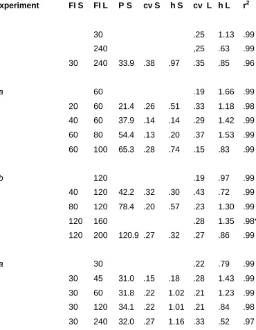
Table 1

Schedule and parameter values from curve fitting conducted on data from

Experiments 1, 2, and 3. FI S, FI L: upper and lower FI value in mixed-FI schedule (in s), single FI values are given as FI L only. P S: peak location, in s, of fitted Gaussian curve corresponding to FI S. cv S, cv L: coefficients of variation of fitted curves. h S, h L: peak heights (responses/s) of fitted curves.

r2: proportion of variance accounted for by the curve fit.

---Experiment FI S FI L P S cv S h S cv L h L r2

1 30 .25 1.13 .99

240 ,25 .63 .99

30 240 33.9 .38 .97 .35 .85 .96

2a 60 .19 1.66 .99

20 60 21.4 .26 .51 .33 1.18 .98

40 60 37.9 .14 .14 .29 1.42 .99

60 80 54.4 .13 .20 .37 1.53 .99

60 100 65.3 .28 .74 .15 .83 .99

2b 120 .19 .97 .99

40 120 42.2 .32 .30 .43 .72 .99

80 120 78.4 .20 .57 .23 1.30 .99

120 160 .28 1.35 .98*

120 200 120.9 .27 .32 .27 .86 .99

3a 30 .22 .79 .99

30 45 31.0 .15 .18 .28 1.43 .99

30 60 31.8 .22 1.02 .21 1.23 .99

30 120 34.1 .22 1.01 .21 .84 .98

(28)

3b 15 300 21.7 .57 .39 .21 .52 .96

30 300 34.8 .40 .43 .39 .19 .97

45 300 50.9 .33 .79 .24 .69 .97

60 300 66.2 .32 .63 .26 .42 .97

75 300 83.1 .33 .50 .32 .43 .96

(29)

References

Beam, J.J., Killeen, P.R., Bizo, L.A., & Fetterman, J.G. (1998). How temporal

context affects temporal production and categorization. Animal

Learning and Behavior, 26, 388-396.

Brown, S.W., & West, A.N. (1990). Multiple timing and the allocation of

attention. Acta Psychologia, 75, 103-121.

Catania, A.C., & Reynolds, G.S. (1968). A quantitative analysis of responding

maintained by interval schedules of reinforcement. Journal of the

Experimental Analysis of Behavior, 11, 327-383.

Church, R.M., & Gibbon, J. (1982). Temporal generalization. Journal of

Experimental Psychology: Animal Behavior Processes, 8, 165-186.

Church, R.M., Meck, W.H., & Gibbon, J. (1984). The application of scalar

timing theory to individual trials. Journal of Experimental Psychology:

Animal Behavior Processes, 20, 135-155.

Dews, P.B. (1978). Studies on responding under fixed-interval schedules of

reinforcement: II: The scalloped pattern of the cumulative record.

Journal of the Experimental Analysis of Behavior, 29, 67-75.

Gibbon, J., & Church, R.M. (1990). Representation of time. Cognition, 37,

23-54.

Gibbon, J., Church, R.M., & Meck, W. (1984). Scalar timing in memory. In

J.Gibbon and L. Allan (Eds.), Annals of the New York Academy of

Sciences, 423: Timing and time perception, (pp. 52-77). New York:

(30)

Herrnstein, R.J. (1970). On the law of effect. Journal of the Experimental

Analysis of Behavior, 13, 243-266.

Killeen, P.R. & Fetterman, G.J. (1988). A behavioral theory of timing.

Psychological Review, 95, 274-295.

Killeen, P.R., Hall, S., & Bizo, L.A. (1999). A clock not wound runs down.

Behavioural Processes, 45, 129-139.

Leak, T.M., & Gibbon, J. (1995). Simultaneous timing of multiple intervals:

Implications of the scalar property. Journal of Experimental

Psychology: Animal Behavior Processes, 21, 3-19.

Lejeune, H., & Wearden, J.H. (1991). The comparative psychology of

fixed-interval responding: Some quantitative analyses. Learning and

Motivation, 22, 84-111.

Lejeune, H., Cornet, S., Ferreira, J., & Wearden, J.H. (1998). How do

mongolian gerbils (Meriones unguiculatus) pass the time? Adjunctive

behavior during temporal differentiation in gerbils. Journal of

Experimental Psychology: Animal Behavior Processes, 24, 325-334.

Lowe, C.F., Harzem, P., & Spencer, P.T. (1979). Temporal control of behavior

and the power law. Journal of the Experimental Analysis of Behavior,

31, 333-343.

Machado, A. (1997). Learning the temporal dynamics of behavior.

Psychological Review, 104, 241-265.

Machado, A., & Guilhardi, P. (2000). Shifts in the psychometric function and

their implications for models of timing. Journal of the Experimental

(31)

Penney, T.B., Gibbon, J., & Meck, W.H. (2000). Differential effects of auditory

and visual signals on clock speed and temporal memory. Journal of

Experimental Psychology: Human Perception and Performance, 26,

1770-1787.

Roberts, S. (1981). Isolation of an internal clock. Journal of Experimental

Psychology: Animal Behavior Processes, 7, 242-268.

Schneider, B.A. (1969). A two-state analysis of fixed-interval responding in the

pigeon. Journal of the Experimental Analysis of Behavior, 12, 667-687.

Skinner, B.F. (1938). The behavior of organisms. New York:

Appleton-Century-Crofts.

Staddon, J.E.R., & Higa, J. (1999). Time and memory: Towards a

pacemaker-free theory of interval timing. Journal of the Experimental Analysis of

Behavior, 71, 215-251.

Wearden, J.H. (1999). "Beyond the fields we know...": Exploring and

developing scalar timing theory. Behavioural Processes, 45, 3-21.

Whitaker, J.S. (1980). Temporal control of animal operant performance.

(32)

Figure legends

Figure 1. Response rates versus elapsed time in the interval from FI 30 s

(upper panel), FI 240 s (center panel), and the FI 240-s intervals of

mixed FI 30 s FI 240 s (bottom panel). Data points are shown as

unconnected filled circles, and the best fitting Gaussian or

2-Gaussian function (see text for details) is shown as a line. Parameter

values for the curve fit are given in Table 1.

Figure 2. Data from the longer components of mixed-FI conditions of

Experiment 2a. Other details as Figure 1.

Figure 3. Data from mixed-FI conditions of Experiment 2b. Other details as

Figure 1.

Figure 4. Data from mixed-FI conditions of Experiment 3a. Other details as

Figure 1.

Figure 5. Data from mixed-FI conditions of Experiment 3b. Other details as

Figure 1.

Figure 6. Upper panel: Peak location (in s) of the Gaussian curve associated

with FI S in the mixed-FI schedules used in Experiments 1 to 3,

plotted against FI S value in s. Lower panel: Number of instances

where the peak height at FI S was greater than at FI L (or lower).

Data are group by L/S ratio (>= 4 or < 4).

Figure 7. Upper panel: Coefficients of variation from the Gaussian curves

fitted to data from single and mixed FI schedules used in Experiments

1 to 3, plotted against the programmed rate of reinforcement provided

by the schedules. Lower panel: Coefficients of variation of curves

fitted to the constant component of the mixed FI schedules used in

Experiments 2 and 3, plotted against reinforcement rate for the

schedule.

Figure 8. Ratio of coefficients of variation of curves fitted to FI L and FI S from

(33)

indicate that the coefficient of variation at FI L was greater than that at

FI S; values below 1.0 the reverse. Data are shown separately from

(34)

Author note

The experimental work reported in this thesis was conducted in partial

fulfilment of the requirements for a degree of Ph.D. awarded to the first author

by the then-titled University College of North Wales, Bangor, in 1980. J.S.

Whitaker is currently in the Learning Disabilities Unit University of

Huddersfield, and C.F. Lowe at the School of Psychology, University of

Wales, Bangor. Correspondence concerning this article should be sent to J.H.

Wearden, Department of Psychology, Manchester University, Manchester,

(35)

Elapsed time in interval (s)

0 5 10 15 20 25 30

Responses per second

0.00 0.25 0.50 0.75 1.00 1.25

0 30 60 90 120 150 180 210 240

0.00 0.25 0.50 0.75 1.00

0 40 80 120 160 200 240

0.00 0.25 0.50 0.75 1.00 1.25 1.50

FI 240 s

(36)

0 10 20 30 40 50 60

Responses per second 0.0 0.2 0.4 0.6 0.8 1.0 1.2

0 10 20 30 40 50 60

0 15 30 45 60 75

Responses per second 0.0 0.2 0.4 0.6 0.8 1.0 1.2 1.4 1.6

0 20 40 60 80 100

(37)

0 20 40 60 80 100 120

Elapsed time in interval (s) 0 20 40 60 80 100 120 140 160

Response per second _0.0

0.2 0.4 0.6 0.8 1.0 1.2 1.4 1.6

0 50 100 150 200

(38)

Elapsed time in interval (s) 0 5 10 15 20 25 30 35 40 45

Responses per second 0.00 0.25 0.50 0.75 1.00

0 10 20 30 40 50 60

0 20 40 60 80 100 120

0 60 120 180 240

(39)

Elapsed time in interval (s) 0 50 100 150 200 250 300

Responses per second 0.0 0.2 0.4 0.6

Response per second _0.0

0.2 0.4 0.6

Mixed FI 45 s FI 300 s

Mixed FI 60 s FI 300 s

(40)

L/S ratio

L/S >=4

L/S < 4

Number of instances

0 1 2 3 4 5 6 7 8

FI S higher FI S lower

FI value (s)

0 20 40 60 80 100 120

Peak location (s)

(41)

Programmed reinforcers per hour

0 20 40 60 80 100

Coefficient of variation

0.0 0.1 0.2 0.3 0.4

Experiment 2a Experiment 2b Experiment 3a Experiment 3b

Programmed reinforcers per hour

0 20 40 60 80 100 120

Coefficient of variation

0.0 0.1 0.2 0.3 0.4 0.5

(42)

L/S ratio

0 5 10 15 20

cv(L)/cv(S)

0.0 0.5 1.0

L/S ratio

1.0 1.5 2.0 2.5 3.0