First Passage Times of Diffusion Processes
and Their Applications to Finance
A thesis presented for the degree of
Doctor of Philosophy
Luting Li
Department of Statistics
The London School of Economics and Political Science
United Kingdom
Declaration
I certify that the thesis I have presented for examination for the Ph.D. degree of the London School of Economics and Political Science is solely my own work other than where I have clearly indicated that it is the work of others (in which case the extent of any work carried out jointly by me and any other person is clearly identified in it).
The copyright of this thesis rests with the author. Quotation from it is permitted, provided that full acknowledgement is made. This thesis may not be reproduced without the prior written consent of the author.
I warrant that this authorisation does not, to the best of my belief, infringe the rights of any third party.
Statement of conjoint work
A version of parts of Chapters 3-6 has been submitted for publication in two articles jointly authored with A. Dassios.
Acknowledgements
Just before writing down the words appearing on this page, I sit at my desk on the 7th floor
of the Columbia House, recalling those countless yet enjoyable days and nights that I have spent on pursuing knowledge and exploring the world. To me, the marvellous beauty of this journey is once in a lifetime.
I would like to, first and foremost, express my sincere gratitude to my supervisors Angelos Dassios and Hao Xing, for providing me the opportunity of carrying out my research under their supervisions, for their constant support and the freedom they granted me to conduct my work according to my preferences. Whenever I was struggling on the research, it was Angelos who always pointed me towards the right direction, guided me out of puzzles, and taught me that persistence is the key to success. I am grateful to him for not only offering invaluable academic advice, but also spending time with me having coffees, talking travels, and sharing experiences, which broadened my horizons outside the academic world. I am indebted to Hao as my secondary supervisor for inviting me to the FRTB project which enriched this thesis in the dimension of quantitative risk management. He was more like a friend than a teacher to inspire and encourage me to excel in my work.
Nevertheless, without the enormous help and precious comments from many experts, this thesis would not be presented in its current complete format. I am honoured for Goran Peskir and Luciano Campi being my examiners to give me invaluable suggestions and help in finalising this thesis. In addition, I would like to thank Jos´e A. Scheinkman and Michael Schatz for providing insightful advice on the financial bubble topic. I am grateful to Paul Embrechts, Demetris Lappas, Dirk Tasche, and Ruodu Wang, for their comments on the capital allocation project. I would also like to express my gratitude to the referees and editors from the Applied Probability Journals, the International Journal of Theoretical and Applied Finance, and the Risk Magazine, for their helpful comments and advice on three
Great thanks go to Citigroup for providing the funding which allowed me to undertake my research. Particularly, I would like to express my sincere gratitude to Demetris Lappas, Wei Zhu, and Kevin Jian, for providing me with the opportunity of joining the Citi-LSE programme and gaining industrial experience alongside my research. My special thanks go to Damien Quinn for sharing his knowledge and introducing me a real financial world. I would also like to extend my thanks to Pierre-Yves Casteill, and George Dimitropoulos, for beautiful birthday gifts, offering me all those unforgettable and relaxing times of having drinks, dinners, and going for hiking, etc.
Moreover, I express my sincere gratitude to all the staff and colleagues from the De-partment of Statistics at LSE for providing such a pleasurable environment. Particularly, I would like to thank my neighbour Jos´e M. Pedraza for his constant support in both academic and non-academic aspects. I gratefully acknowledge the helpful discussions from Yan Qu and Junyi Zhang about the research. And I would like to thank Ian Marshall and Penny Montague for their administrative support.
I would like to express my deep friendship to Longjie Jia, Phoenix H. Feng, Cong Liu, Yusong Li, and Yupeng Jiang to share with me all those joy and sadness moments in the past four years in London. I wish to express my gratitude to Shuren Tan, for providing me timely help in Edinburgh. Also, I would like to give my special thanks to my car, for always driving me to office and journey, no matter sunny, raining, or snowing, and never abandoning me on its halfway.
Naturally, I should not forget my teachers who gave me knowledge prior to my doctoral training and those friends who accompanied me though not in this country. I would like to thank my junior high school teacher Haiying Zhou who inspired me to realise the beauty of mathematics; my senior high school teacher Chengsheng Ma who encouraged me to always follow my heart; and my teacher Goran Peskir at the University of Manchester who introduced the stochastic calculus world to me. I would like to express my gratitude to Honghua Qiao, Chao Zhang, and Xuheng Lu, for their encouragement throughout these years.
Abstract
This thesis consists of three submitted papers and one working paper. It begins with the study of asymptotic solutions for the first passage time densities of various diffusion processes, and the thesis ends up with an application of such findings in the area of systematic trading. In between, financial bubbles and the regulatory risk management for the banking industry are studied additionally. The purpose of this thesis is to, by combining probability theory with financial practice, provide quantitative tools for investment decision and risk management.
Chapters 3-5 are reorganised from the first passage time paper [31]. Our research method is mainly based on the potential theory and the perturbation theory. In Chapter 3, a unified recursive framework for finding first passage time asymptotic densities has been proposed. Besides, we prove the convergence of our framework and provide an error estimation formula. Examples related to the Ornstein-Uhlenbeck and the Bessel processes are demonstrated in Chapters 4 and 5, respectively.
The second paper [30] is documented in Chapter 6. It introduces a new diffusion process which is relevant to financial bubbles. During the study of the first passage time, we occa-sionally found that the sample path of the new process coincides with log-price features of bubble assets. In Chapter 6, we show that the new model is a power-exponential transform of the Shiryaev process [116, 117]; and we prove that the model itself, indeed, satisfies var-ious technical requirements for defining a financial bubble [107]. Furthermore, by using our previous framework, we solve the closed-form asymptotic for the model’s first passage time; and according to which, we have made predictions to the burst time of BitCoin.
Chapter 7 is a modified version of the third paper [75]. We consider the risk capital allo-cation issue under the forthcoming regulatory framework, namely theFundamental Review of Trading Book. Apart from studying coherent properties of the new risk measure, we propose
dif-ferent allocated capitals, therefore, impacting on bank’s performance measure and capital optimisation.
Contents
1 Introduction 1
2 Preliminary Definitions and Results 5
2.1 Stochastic Differential Equation . . . 5
2.2 First Passage Time . . . 10
2.3 Inverse Laplace Transform Algorithm . . . 14
2.4 Portfolio Selection, Risk Management and Capital Allocation . . . 17
2.5 Table of Nomenclature . . . 23
2.5.1 Abbreviation . . . 23
2.5.2 Set and Space . . . 24
2.5.3 Probability and Stochastic Process . . . 25
2.5.4 Operation and Operator . . . 26
2.5.5 Function . . . 27
3 Explicit Asymptotics on the First Passage Times of Diffusion Processes 29 3.1 Introduction, Motivation, and Literature Review . . . 29
3.2 Perturbed Dirichlet Problem . . . 32
3.3 Truncation Error and Convergence . . . 34
3.4 Recursion under Frequency Domain . . . 37
Appendix 3.A Alternative Error Estimation . . . 39
Appendix 3.B Probabilistic Representation of p(τN)(t) . . . 40
4 First Passage Time of Ornstein-Uhlenbeck Process 43 4.1 N-th Order Perturbed FPTD . . . 44
4.3 Model Application . . . 53
4.3.1 Extension . . . 53
4.3.2 Alternative Approach for the OU FPTD . . . 55
4.3.3 Numerical Example on Downward OU FPTD . . . 56
Appendix 4.A Proof of Proposition 4.1.1 . . . 60
Appendix 4.B Recursive Polynomial Decomposition and Proof of Lemma 4.1.2 . . 61
Appendix 4.C Further Numerical Result . . . 66
5 First Passage Time of Bessel Process 68 5.1 First Order Perturbed FPTD . . . 69
5.2 Tail Asymptotic and Error Estimation . . . 73
5.3 Numerical Example on Downward BES(1 +) FPTD . . . 78
5.4 Conclusion . . . 80
Appendix 5.A Upward FPTD of BES(1 +) . . . 80
Appendix 5.B Extension to BES(n) . . . 82
Appendix 5.C Lower Boundary of CIR FPTD . . . 84
6 An Economic Bubble Model and Its First Passage Time 87 6.1 Introduction, Motivation, and Literature Review . . . 88
6.2 Stochastic Dynamic, Economic Bubble, and Burst Time . . . 90
6.3 Theoretical Result . . . 95
6.3.1 Existence, Uniqueness and the Strong Markov Property . . . 95
6.3.2 Probability Distribution of{Xt}t≥0 . . . 97
6.3.3 Finiteness of the First Passage Time . . . 103
6.4 First Passage Time of{Xt}t≥0 . . . 105
6.4.1 Solution of the Initial Dirichlet Problem . . . 105
6.4.2 Perturbed Downward FPTD . . . 107
6.5 Model Implementation . . . 112
6.5.1 Model Calibration . . . 113
6.5.2 Numerical Example . . . 115
6.6 Conclusion . . . 124
Appendix 6.A Recursive Solution forc= 0 . . . 124
Appendix 6.C Further Numerical Analysis for {Xt}t≥0 . . . 128
Appendix 6.D First Order Perturbed Upward FPTD . . . 129
7 Capital Allocation under the Fundamental Review of Trading Book 131 7.1 Introduction, Motivation, and Literature Review . . . 132
7.2 Internal Model Capital Charge under FRTB . . . 134
7.2.1 Risk Factor and Liquidity Horizon Bucketing . . . 134
7.2.2 Stress Period Scaling and IMCC . . . 136
7.2.3 Property of IMCC . . . 138
7.3 Capital Allocation . . . 140
7.3.1 Euler Allocation . . . 141
7.3.2 Constrained Aumann-Shapley Allocation . . . 143
7.3.3 The Second Step Allocation . . . 146
7.3.4 Extension . . . 147
7.4 Simulation Analysis . . . 148
7.4.1 Positive Correlation . . . 148
7.4.2 Hedging . . . 150
7.4.3 Allocation with Scaling Adjustment . . . 152
7.5 Conclusion . . . 154
Appendix 7.A Proof of Lemma 7.2.2 . . . 155
Appendix 7.B Proof of Proposition 7.3.4 . . . 156
Appendix 7.C Proof of Lemma 7.3.6 . . . 156
Appendix 7.D Proof of Proposition 7.3.8 . . . 158
Appendix 7.E Proof of Proposition 7.3.12 . . . 158
8 Application in Systematic Trading 160 8.1 Introduction, Motivation, and Literature Review . . . 160
8.2 Trading Signal Identification via the First Passage Time . . . 163
8.2.1 Executable Strategy and the TSI . . . 164
8.2.2 Long-Short Strategy by FPT . . . 168
8.2.3 Discussion . . . 170
8.3 Numerical Verification . . . 172
8.3.2 Trading Strategy Illustration . . . 175
8.3.3 Backtest on Simulated Portfolio . . . 178
8.3.4 Risk Management and Capital Allocation . . . 181
8.4 Conclusion . . . 184
Appendix 8.A China Stock Market Exercise . . . 184 Appendix 8.B Further Illustration on the Simulation Exercise and the FPT-TSI . 186
List of Figures
4.1 FPTD of OU process . . . 58
4.2 Relative errors to iv) . . . 58
4.3 FPTD of OU process for general case . . . 59
4.4 Relative error to i) for general case . . . 59
4.5 OU left tail density forl=θ. . . 66
4.6 OU left tail error forl=θ . . . 66
4.7 OU left tail density forl6=θ. . . 67
4.8 OU left tail error forl6=θ . . . 67
5.1 Bessel density with = 0.1, x= 0.7, l= 0.1 . . . 79
5.2 Bessel density error with = 0.1, x= 0.7, l= 0.1 . . . 79
5.3 Bessel left tail density . . . 79
5.4 Bessel left tail relative error . . . 79
5.5 Upcrossing FPTD of BES(1.5). = 0.5, x= 1.8. Left figure, 20% upcrossing (a= 2.16); right figure, 100% upcrossing (a= 3.6) . . . 82
5.6 Upcrossing FPTD of BES(0.5). =−0.5, x= 1.8. Left figure, 20% upcrossing (a= 2.16); right figure, 100% upcrossing (a= 3.6) . . . 82
5.7 Upcrossing probability of BES(3). = 2, x= 1.8. Left figure, 20% upcrossing (a= 2.16); right figure, 100% upcrossing (a= 3.6) . . . 83
5.8 Upcrossing probability of BES(6.5). = 5.5, x = 1.8. Left figure, 10% upcrossing (a= 1.98); right figure, 20% upcrossing (a= 2.16) . . . 84
6.1 Function plots ofe−2αXt withα= 0.1,0.5,1,2. Green zone: positive drift; red
zone: negative drift . . . 93 6.2 Sample path of eXt in 1 year time. Parameters are chosen as α = 2, = 0.1,
c= 0.5, X0 = 0 anddt= 2601 . . . 93
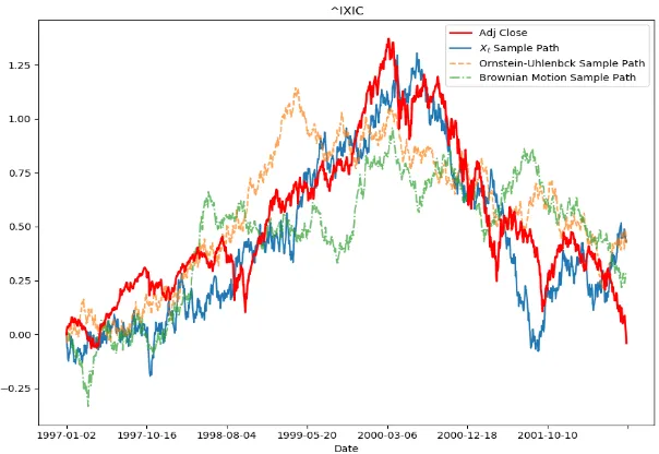
6.3 Model calibration comparisons for NASDAQ index (US ticker symbol ˆIXIC) from 1997-01-02 to 2003-12-30. Red curve: historical adjusted log-price; blue curve: the best of 1,000 simulations from{Xt}t≥0; orange curve: the best of
1,000 simulations from OU process; green curve: the best of 1,000 simulations
from DBM. Calibration parameters,{Xt}t≥0 : (ˆ,α,ˆ σ,ˆ ˆc) = (0.39,0.23,0.43,0.73); OU :
(ˆκ,µ,ˆ σˆ) = (0.47,1.09,0.31); BM : (ˆµ,σˆ) = (0.25,0.31). The data source is from Yahoo Finance . . . 118 6.4 Algorithm 1 illustration based on ˆIXIC and 10,000 paths simulation starting
fromX0 = ˆXt3 . Green zone indicates regime I, the displacement stage; yellow
zone indicates regime II, the boom stage; red zone indicates regime III, the euphoria & profit taking stages. Blue curve shows the historical data used for calibration. Red curve, covered by shadowed region, shows the historical data aftert3. The shadowed region plots 10,000 simulation paths . . . 118
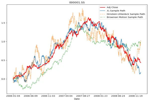
6.5 Model calibration comparisons for Shanghai Stock Exchange Composite in-dex (US ticker symbol SSEC, China ticker symbol 000001.SS) from 2006-01-04 to 2008-12-31. Red curve: historical adjusted log-price; blue curve: the best of 1,000 simulations from {Xt}t≥0; orange curve: the best of 1,000
simula-tions from OU process; green curve: the best of 1,000 simulasimula-tions from DBM. Calibration parameters, {Xt}t≥0 : (ˆ,α,ˆ σ,ˆ cˆ) = (0.32,0.14,0.56,0.70); OU :
(ˆκ,µ,ˆ σˆ) = (3.30,0.97,1.20); BM : (ˆµ,σˆ) = (0.44,0.33). The data source is from Yahoo Finance . . . 120 6.6 Algorithm 1 illustration based on 000001.SS and 10,000 paths simulation
start-ing from X0 = ˆXt3. Green zone indicates regime I, the displacement stage;
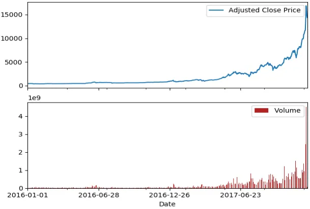
6.7 Bitcoin daily price and trading volume from 2016-01-01 to 2017-12-10. The data source is from Yahoo Finance . . . 121 6.8 BitCoin closing price between 2017-12-10 and 2018-01-12. The probabilities of
different thresholds are reported in Table 6.1 . . . 123 6.9 Density plot with = 0.1, α= 0.5, c= 0.2, σ = 0.5, x= 0.7, l= 0.2 . . . . 129 6.10 Error plot with = 0.1, α= 0.5, c= 0.2, σ= 0.5, x= 0.7, l= 0.2 . . . 129 6.11 Left tail density . . . 129 6.12 Left tail density error . . . 129 6.13 Upcrossing FPTD of the bubble process. = 0.1, α = 0.5, c = 0.3, σ =
0.4, x = 1.5. Left figure, 20% upcrossing (a = 1.8); right figure, 100% up-crossing (a= 3). . . 130
7.1 Euler allocation of IMCC (Euler FRTB ES), CAS allocation of IMCC (CAS FRTB ES), and Euler allocation of regular ES (Euler Reg ES). Upper-left panel: scenario (i); upper-right panel: scenario (ii); bottom-left panel: scenario (iii); bottom-right panel: scenario (iv). Each panel presents the percentage of allocation to different ˜X(i, j). The total capital charges are reported in Table 7.1 . . . 149 7.2 Kernel smoothed allocations . . . 150 7.3 Allocations of IMCC and regular ES for portfolios with hedging components.
Left panel: hedging structure (i); middle panel: hedging structure (ii); right panel: hedging structure (iii). Each panel presents the percentage of allocation to different ˜X(i, j). The total capital charges are reported in Table 7.2 . . . . 152 7.4 Histograms and kernel densities for FRTB allocations and regular ES
allo-cation. Extreme allocations: i) Euler FRTB ES: left end, -5.50%; right end: 6.32%; ii) CAS FRTB ES: left end, -4.69%; right end: 5.39%; iii) Euler Regular ES: left end, -11.19%; right end: 11.83% . . . 153
8.1 Simulated portfolio paths (normalised) with equal weights across different assets175 8.2 First stage signal illustration of portfolio #542. Blue and orange curves refer
to the upcrossing probability and the difference between upcrossing and down-crossing probabilities. Red solid line indicates αu and red dashed line plots
8.3 One stage backtest of portfolio #542 between t= 1 andt= 1 + 2/12. Green curves marked by star symbols demonstrate the selected paths that attain the 20% target increase; green curves with no marks show the selected paths but which are held until t=1+2/12. Grey paths are for unchosen assets . . . 177 8.4 One-year backtest of portfolio #542 betweent= 1 and t= 2. Green and blue
curves refer to two schemes of the FPT-TSI; red and purple curves plot the performances of global portfolios . . . 179 8.5 Sharpe ratio histograms for one-year backtests of 1,000 simulated portfolios . 181 8.6 Portfolio value and different risk metrics of portfolio #542 between year 1 and
year 2. The left panel presents the FPT-TSI portfolio and the right panel shows the global portfolio. Both portfolios are of Markowitz types. And in both graphs, blue curve indicates the normalised portfolio values, green curve plots the FRTB IMCCs; red and purple curves represent the VaR and the ES metrics, respectively . . . 182 8.7 Risk metric proportions to the total portfolio value. Left panel: FPT-TSI
portfolio; right panel: global portfolio . . . 182 8.8 Annually averaged risk contributions of each RF-LH bucket for the FPT-TSI
and the global portfolios . . . 183 8.9 China stock market statistics (historical time-series) for stocks which have more
than 20% increase within 2 months time. Left panel: in terms of absolute stock numbers; right panel: in terms of ratios in the total stock amounts. Yellow region: accounting for the Shanghai market only; blue region: total numbers of Shanghai and Shenzhen markets . . . 184 8.10 Backtest of China stock market between 2007-2018. Left panel: normalised
8.12 Initial state probabilities for portfolio #542 of upward- and downward-hittings in 2 months time (betweent0 = 0 andt1= 2/12). Left panel: upward hitting;
right panel: downward hitting. The underlying processes for each asset class are specified as: commodity - OU, credit - Bubble; foreign exchange - OU; interest rate - CIR; equity - DBM. The y-axis refers to the hitting probability and the x-axis represents the number of asset. There are 100 assets under each class and in total 500 assets . . . 187 8.13 First stage signal illustration (Equation (8.5)) of portfolio #542. Blue and
orange curves refer to the upcrossing- and the downcrossing-probabilities (mu
and ml, respectively). Red solid line indicatesαu and red dashed line plots αl 187 8.14 Blue curve: success rate of attaining 20% increase target; green curve:
List of Tables
6.1 BitCoin imminent risk prediction between 2017-12-10 and 2018-01-12. Columns 1-4 correspond to the percentage of price drop, dropped price Pl, probability
of the lowest pricePt∗ (min0≤s≤tPs), and the relative error in density peaks . 122
7.1 FRTB IMCC v.s. regular ES . . . 148
7.2 FRTB IMCC v.s. Regular ES . . . 151
7.3 Ratios between the FRTB-ES using the reduced set and the full set . . . 154
7.4 Percentages of allocations with and without stress-scaling adjustment using different reduced factor sets. Columns labeled adjustment report allocations using (7.22), columns labeled without adj report allocation using (7.15). The total IMCC are the same in both methods: IMCC(Set A)=11.55; IMCC(Set B)=3.14 . . . 154
8.1 Model choices and numbers of simulated paths in different regimes . . . 174
8.2 Formulae of perturbed FPTDs for each model . . . 176
8.3 Statistics of one step backtest through 1,000 simulations . . . 178
8.4 Statistics of one-year backtest on portfolio #542 . . . 180
8.5 Sharpe ratio statistics for one-year backtests of 1,000 simulated portfolios . . 181
Chapter 1
Introduction
The majority of this thesis is technical discussions about the first passage time. Apart from its theoretical results which are based on time-homogeneous diffusion processes, this thesis also considers applications in economic bubble forecasting and trading signal identification. Simultaneously, a separate topic about the regulatory risk capital allocation is presented. From the financial practice aspect, this thesis could be regarded a self-contained material relevant to investment decision and risk management.
This chapter provides an overview of the thesis, where general motivations of the research and an outline of following chapters are explained. On its whole, this thesis contains 4 different topics. Later for each topic, the background introduction, motivation, and literature review are documented separately.
Our research about the first passage time was originally motivated by the pricing and hedging problems in credit derivatives. According to R.C. Merton’s earlier work [88], and followed by the extensions from F. Black and C. Cox [15], and many others (cf. [108] for a brief summary), the stochastic barrier crossing problem has attracted much attention in the area of thestructural modelling approach. On the other hand, point processes are usually used in the intensity-based modelling approach for credit risk (cf. A. Dassios and H. Zhao [37]). And those processes would require the information about first passage time distributions. Therefore, calculations involved in but not limited to credit risk/derivative pricing, would be benefited from by knowing the closed-form densities of first passage times.
methods of studying the first passage time distribution is to employ the killed version po-tential theory (cf. G. Peskir [101]). By solving ODEs with Dirichlet-type boundaries, such a theory generates Laplace transforms of first passage times. But the problem comes from the fact that most those transforms are given by ratios of special functions, and which are rarely known of having closed-form inverses. In order to simplify the problem, we further adopt the perturbation theory. The perturbation technique was initially applied in the area of quan-tum physics [110], while our inspiration for using it is from the works about the stochastic volatility modelling [45] and theParisian option pricing [35].
In the first topic of this thesis, we present a recursive framework for solving the first pas-sage time asymptotics of time-homogeneous diffusion processes. The research began with the perturbation analysis on the Ornstein-Uhlenbeck and Bessel models. After gaining successes from these two processes, plus our observations of commonalities in their perturbed ODEs, we realised that the perturbation mechanism might be effective to a more general class of diffusion processes. This motivates us to deduce a unified framework for solving the constant barrier crossing problem in an asymptotic manner. However, the perturbation technique in general would not provide error estimation results. Though under certain circumstances our numerical exercises have shown that perturbed densities are accurate, we want to fur-ther understand the error terms remained in the perturbed ODEs. In the end, by referring again to the potential theory, we were able to derive an error estimation formula. And as a by-product of this formula, we have proved that under theL1-boundedness condition, the perturbed density iso(N)-accurate, where N is the truncation order in the recursion system andis the perturbation parameter.
between the new model and the financial bubbles. Later by extending the original SDE with a negative drift parameter, we have demonstrated that our model is a well-defined bubble process1 [107]. From the investor behaviour point of view, the new model explains the posi-tive feedback mechanism (pro-cyclicality)as well. At the end of this research, we applied our previous perturbation framework and made predictions to the BitCoin price collapse time.
The third topic is independent2 to previous discussions about the first passage time. It focuses on financial regulation and provides two risk capital allocation schemes under the Fundamental Review of Trading Book. In January 2016, the Basel Committee on Banking
Supervision overhauled the quantitative methodologies for bank’s minimum capital require-ments [12]; according to which, banks need to reevaluate their capital efficiency and optimise their capital structures. Within this context, the industry is awaiting a tailored allocation scheme to the new regulation. And this research responds to such a need. Although there is no sophisticated mathematics in this topic, two main challenges arise from the conceptual and computational aspects. In this study, we established a mathematical framework translated from the original regulation document. Based on this framework, we analysed the coherent properties of the new regulatory risk metric and deduced two allocation schemes by using the Euler approach and the constrained Aumann-Shapley approach. Numerical exercise shows that our new methods could effectively reflect bank’s capital structure, meanwhile, compu-tationally they are no more complex than the current VaR-based allocation methods. In the end, evidence from our work indicates that the allocation results could be used in the future capital optimisation problem.
The last topic of this thesis summarises some of our thinkings about systematic trading. The motivation for conducting this research comes from two dimensions. On the one hand, inspired by the Ornstein-Uhlenbeck process and its first passage time in pairs trading [47], we want to generalise this trading idea to various diffusion processes with clear economic mean-ings. On the other hand, considering that our third and first two topics are distinct in theory, in order to maintain the integrity of this thesis, we include Chapter 8 to illustrate how the theoretical parts of this thesis can be applied in a whole investment life cycle: from decision making to risk evaluation. In this topic, we discuss thetrading signal identification problem. The ‘identification’ here refers to an extra step prior to the portfolio weight allocation (cf.
1And mathematically, it is closely related to the Shiryaev process [116, 117]. 2
themodern portfolio theory [83, 84]). During this step, quantitative criteria associated with executable strategies should be specified; and such criteria constitute the decision metric for portfolio investment. Following this thinking, we demonstrate how the probability of the first passage time can be adopted as a trading signal identification metric. And we use simulated portfolios to show that the investment performance could be evidently enhanced under the new strategy3. In addition, as an illustration of the risk capital allocation topic, we report the risk capital and its allocated numbers in our simulated investments.
We now conclude this chapter by outlining the structure of the thesis. Topic 1 is dis-tributed in Chapters 3-5. And Topics 2-4 are documented separately through Chapters 6-8. In general, each topic has its own abstract, introduction, and conclusion. And in each chap-ter, apart from its main body, we may also include separate appendices to record supporting materials or less-relevant but interesting findings. Based on these principles, the rest of this thesis is organised as follows.
In Chapter 2, we introduce notations, concepts, and major theorems, which are used throughout this thesis. Chapter 3 presents the unified recursive framework, together with its convergence results, for solving the first passage times of time-homogeneous diffusion pro-cesses. Chapter 4 demonstrates the application of our framework on the Ornstein-Uhlenbeck process. In this chapter, we provide the N-th order results of perturbed densities, their tail asymptotics, and the proof for the first order convergence. Chapter 5 is the same in structure as Chapter 4, but discussions are based on the first order results of the Bessel process. Note that, an abstract and an introduction of Topic 1 are given at the beginning of Chapter 3, and the conclusion is provided at the end of Chapter 5. In Chapter 6, we summarise our findings in the financial bubble model. This chapter can be read in two parts. The first part conducts stochastic analysis about the model itself; and the second part calculates its first passage time. Chapter 7 reports our third topic about the risk capital allocation. And Chapter 8 illustrates our thoughts about systematic trading, which, meantime, can be regarded as an application summary of the technical parts of this thesis. In the end, Chapter 9 concludes this thesis and highlights further works.
Chapter 2
Preliminary Definitions and Results
This chapter reviews major theoretical results that are relevant to the work of this thesis. In order to accommodate notations and settings in this thesis, theorems in this chapter could be modified versions from classical conclusions. In general, apart from where it is mentioned, there is no new material in this chapter.
This chapter is organised into three parts. Sections 2.1, 2.2, and 2.3 form the first part. In this part, we review classical theorems in stochastic analysis and numerical methods for the inverse Laplace transform. These results will be referred to later by Chapters 3, 4, 5, and 6. In the second part, Section 2.4, we introduce relevant concepts in portfolio selection, risk management, and capital allocation. The second part can be seen as a partial literature review of Chapters 7 and 8. The last section (Section 2.5) of this chapter summarises notations that will be used throughout this thesis, and it forms the last part of this chapter.
2.1
Stochastic Differential Equation
Consider a filtered probability space Ω,F,{Ft}t≥0,P
which satisfies the usual condi-tions (completeness and right-continuity) and is generated by a (standard) Brownian motion
{Wt}t≥0. LetDbe an open interval on the real lineR, and on which we define two continuous
measurable functionsµ(·) andσ(·). Given the settings above, the stochastic process{Xt}t≥0
with the following SDE
is Markovian and has a continuous path. Let C2 be the short for the C2(D)-space1. For
f ∈C2, denote the infinitesimal generator of {Xt}t≥0 by
Af(x) := lim
t↓0
Exf(Xt)−f(x)
t , x∈D, (2.2)
whereEx·:=E[·|F0] =E[·|X0 =x] by the Markov property. If the limit on the right-hand
side of (2.2) exists, we say {Xt}t≥0 is a 1-dimensional time-homogeneous diffusion process.
Correspondingly, the infinitesimal generator of{Xt}t≥0 is explicitly given by
Af(x) =µ(x)∂xf(x) +
1 2σ
2(x)∂
xxf(x). (2.3)
Example 2.1.1(Brownian Motion). Let{Wt}t≥0 defined onRbe a Brownian motion, then
its infinitesimal generator is given by
Gf(x) = 1
2∂xxf(x). (2.4)
The first concept related to our work is theexistenceanduniqueness of solutions to SDEs. Intuitively, the existence of a unique solution guarantees that we can depict the sample path of{Xt}t≥0by using its specified SDE and a realisation of a Brownian motion path. In Chapter
6 of this thesis, a new stochastic process has been introduced. And the first thing we should be clear is that whether the process possesses a unique strong solution. The answer is given by the following theorem.
Theorem 2.1.2(Existence, Uniqueness, and Square-Integrability). LetK >0be a constant, and assume thatµ(·), σ(·) satisfy the conditions
|µ(z)−µ(y)|+|σ(z)−σ(y)| ≤K|z−y|, (2.5)
µ(y)2+σ(y)2≤K2(1 +y2), (2.6)
where y, z ∈D. If E|X0|<+∞, then there exists a unique, continuous and adapted process
{Xt}t≥0 which is a strong solution of SDE (2.1). Moreover, {Xt}t≥0 is square-integrable,
i.e.,∀T >0 and 0≤t≤T, there exists a constant C:=C(K, T), such that
E|Xt|2≤C(1 +X02)eCt.
Proof. Please refer to [68, Theorems 2.5 & 2.9, Section 5.2].
On the other hand, as a part of the study of the Markov process, very often we are inter-ested in thetransition density of {Xt}t≥0. Our main research tool is using the Kolmogorov
Forward equation (Fokker-Planck equation). Define the adjoint operator of A (in Equation (2.3)) as
A∗g(u) :=−∂u(µ(u)g(u)) +
1 2∂uu(σ
2(u)g(u)), g∈C2 and u∈D. (2.7)
According to classical probability theory, thefixed time transition density, denoted by
px(u, t) := P
x(Xt∈du)
du , t >0, wherePx(·) :=P(·|X0 =x), (2.8)
solves the following Fokker-Planck equation:
A∗px(u, t) =∂tpx(u, t). (2.9)
The initial condition is specified bypx(u,0) =δx(u), whereδx(u) is theDirac delta function.
In addition, by finding the infinite time distribution, we can further check whether a given process is stationary. Denote the stationary distribution by (note that such a distribution should be independent of the initial statex):
p(u) := lim
t↑+∞px(u, t).
Then substitute∂tp(u) = 0 into (2.9),p(u) solves
A∗p(u) = 0, (2.10)
given the full-integration conditionR
Dp(u)du= 1 holds.
process should be finitea.s. For a given diffusion process, the following two theorems can be used to check if these two technical conditions are satisfied.
Theorem 2.1.3 (Strong Markov Property). If conditions (2.5) and (2.6)are satisfied, then the solution {Xt}t≥0 to SDE (2.1) is strong Markov.
Proof. Since µ(·) and σ(·) are continuous on D, therefore they are bounded on compact subsets of D⊆R. Combine the Lipschitz continuity and linear growth conditions, {Xt}t≥0
then has a unique strong solution. According to [68, Theorem 4.20, Section 5.4], we conclude that{Xt}t≥0 is strong Markov.
The finiteness of FPT can be justified by that {Xt}t≥0 is a recurrent process. More
precisely, a recurrent Markov process means, with probability 1 that the process will hit any predefined crossing level in its domain. Before stating the second theorem, we introduce the following notations related to the scale function. Define the left and right boundaries of D
byl and r, respectively, i.e.
∂D ={l, r}, with − ∞ ≤l < r ≤+∞. (2.11)
For the functionsµ(·) and σ(·), we introduce thenon-degeneracy and local-integrability con-ditions by:
σ2(y)>0, ∀y∈D; (2.12)
Z y+δ
y−δ
1 +|µ(z)|
σ2(z) dz <+∞, ∀y, y+δ, y−δ ∈Dwith some δ >0. (2.13)
Consider a fixed numberc∈D, define
s(y) :=
Z y
c
exp
−2
Z ξ
c
µ(ζ)dζ σ2(ζ)
dξ, y∈D (2.14)
to be the scale function of{Xt}t≥0. Then,
Theorem 2.1.4(Recurrent Process). Under assumptions (2.12) and (2.13), if
lim
y↓ls(y) =−∞, and limy↑rs(y) = +∞,
Proof. Please refer to [68, Proposition 5.22, Section 5.5].
Example 2.1.5 (Ornstein-Uhlenbeck Process). Let{Xt}t≥0 defined on Rbe the
Ornstein-Uhlenbeck (OU)process with
µ(Xt) =(θ−Xt), σ(Xt) =σ, (2.15)
where > 0 is the mean-reversion rate, θ ∈ R is the equilibrium level, and σ > 0 is the instantaneous volatility. The OU process is a strong Markov process which possesses a unique strong solution. Moreover,{Xt}t≥0 is recurrent and the stationary distribution is Gaussian,
with meanθ and variance σ22.
Now we introduce the last theorem of this section, known as the time-change technique for martingales. In practice, for the purpose of simplifying calculations, we usually want to reduce eitherµ(·) orσ(·) to known forms. For example, one can use theGirsanov theorem to remove the drift term; or, as an alternative, thestochastic clock introduced in below enables us to simplify the diffusion term.
Theorem 2.1.6 (Dambis, Dubins & Schwarz Theorem). Let {Mt}t≥0 be a continuous
local-martingale generated by a completed Brownian filtration FW. If lim
t↑+∞hMit = +∞ a.s.,
then there exists a Brownian motion {Bt}t≥0 which is adapted to FB, and such that
Mt=BhMit a.s., 0≤t <+∞.
Proof. Please refer to [68, Theorem 4.6, Section 3.4].
In the theorem above, it should be noticed that{Bt}t≥0and{Mt}t≥0are from two different
but interconnected filtrations. In fact, for 0≤s <+∞, define the stopping time
T(s) = inf{t≥0 :hMit> s},
thenFB is given by the original filtration but which is indexed on the stochastic clockT(s):
Example 2.1.7(Cox-Ingersoll-Ross Process). Let{Xt}t≥0 defined onR+∪ {0}be the
Cox-Ingersoll-Ross (CIR)process with2
µ(Xt) =(θ−Xt), σ(Xt) =σ
p
Xt. (2.16)
According to [50], {Xt}t≥0 can be expressed via a squared Bessel process {Yt}t≥0. More
precisely,
Xt=e−tYσ2 4(et−1)
, (2.17)
where
dYt=
4θ σ2 dt+ 2
p
YtdWt. (2.18)
If we further consider the transform Zt = √
Yt, then by definition and the Itˆo’s lemma, {Zt}t≥0 is the n-dimensional Bessel process (BES(n)) with SDE
dZt=
n−1 2Zt
dt+dWt, (2.19)
wheren= 4σθ2.
2.2
First Passage Time
The FPT, known also as the first hitting time, describes the randomness of time for which a stochastic process would spend to enter or exit a specific state. Let {Xt}t≥0 defined on
D solve SDE (2.1), and assume that {Xt}t≥0 satisfies various conditions (especially with
continuous path) that we have discussed in Section 2.1. Denote thecomplement set ofD in
Rby Dc:=R\D. Then,
τ := inf{t≥0 :Xt∈Dc} (2.20)
defines astopping time. We follow the convention that inf∅= +∞.
In particular, for some constant a ∈ R and D = (a,+∞), Equation (2.20) defines the
single-side downward FPT of {Xt}t≥0. Similarly, by letting D = (−∞, a), we say τ is the
single-side upward FPT of {Xt}t≥0.
The FPT itself is a random variable. In order to find its probabilistic description, we
2
start with solving the corresponding Laplace Transform (LT) of the FPT density (FPTD). Roughly speaking, there are two major ways of finding the LT of τ, namely the martingale approachand theMarkov approach. Although derivations are different in these two methods, in the end, they both link the LT to the Dirichlet-typeBoundary Value Problem (BVP). In this section, we follow [101] and focus on theoretical settings under the Markov approach. The second step, finding the FPTD by inverting the LT, will be discussed in Section 2.3 and in other chapters of this thesis.
According to our assumptions, {Xt}t≥0 is adapted to a Brownian filtration and has a
continuous path. Therefore, the FPTs to either an open interval or its closure are equala.s. (i.e. the boundary ofDis regular). W.l.o.g., we define
P(τ = 0|X0∈Dc) = 1. (2.21)
And as a result of (2.21), we can also show that
P(τ >0|X0∈D) = 1.
For a single-side level crossing problem, if we consider the extended real set, then the complement set ofD will include{−∞,+∞}. In this case, since {Xt}t≥0 is well-defined and
should not explode, so we can further require
P(τ = +∞|X0 ∈ {−∞,+∞}) = 1. (2.22)
On the other hand, we have also assumed that{Xt}t≥0 is a recurrent process. Therefore, by
definition, for the process starting inD, we have
P(τ <+∞|X0 ∈D) = 1.
Consider that{Xt}t≥0 is strong Markov. Based on our notations and assumptions above,
we have the following result.
β∈C+), let f(x)∈C2 be the unique solution to the killed version Dirichlet problem:
Af(x) =βf(x), x∈D, (2.23)
with boundary conditions
f(∂D) =V , x∈∂D, (2.24)
where ∂D is defined on the extended real set and V is determined by conditions (2.21) and (2.22). Then
f(x) =Ex
h
e−βτi. (2.25)
Proof. Please refer to [101, Section 7.1].
There are a few points should be noticed on Theorem 2.2.1. First, even though we write
f(x) as a function of x ∈ D∪∂D, in fact, it also depends on the complex parameter β. Therefore, in this thesis, we will use eitherf(x), or
f(x, β), (2.26)
to refer to the LT of τ (Equation (2.25)). And correspondingly, the C2 set in the theorem above should be understood as the set of functions defined on (D∪∂D)×C+, and which
are twice differentiable on the first argument and first order differentiable on the second argument, i.e.
C2 :=C2,1 (D∪∂D)×C+. (2.27)
Secondly, in the theorem above, we do not require the domain D to be bounded (actually for a single-barrier problem it is not); however, the functionf(x) is indeed bounded. To see this, consider the boundary condition (2.22), it impliesf(x) = 0 for x=±∞and β ∈C+.
The conclusion from Theorem 2.2.1 is very similar to that from theFeynman-Kac theorem; while for the second theorem, when we apply it on the stopping time, extra boundedness conditions on τ should be taken into account. Therefore, using the Feynman-Kac theorem would introduce further technical discussions in our work. In fact, by digging into the proof details3 in [101, Section 7.1], one can find that the connection between ODE (2.23) and
3
the probabilistic representation (2.25) is derived from the mean-value property of harmonic functions. And the idea behind the mean-value property is very akin to the concept of ‘fair
game’ under the martingale settings. As a quick remark, we emphasise that the reason we choose the Markov version is due to its simplicity in technical treatments.
Example 2.2.2 (Single-Side FPT of Brownian Motion). Let
Xt=x+Wt, t≥0,
be a Brownian motion starting from x∈R. Then the LT for the FPT of {Xt}t≥0 hittinga,
is given by [18, Equation 2.0.1, Page 198]:
f0(x, β) =e−
√
2β|x−a|. (2.28)
Moreover, the inverse transform (i.e. the FPTD) is given by
p(0)τ (t) = |√x−a|
2πt3e
−(x−2ta)2. (2.29)
As an extension to (2.25) and Theorem 2.2.1, in the last part of this section, we introduce the Dirichlet problem with an extra Lagrange functional.
Theorem 2.2.3 (Killed Version Dirichlet-Type BVP with Lagrange Functional). Let l(x) defined on D be continuous, and let f(x) ∈ C2 be the unique solution to the killed version Dirichlet problem with Lagrange functionall(x):
Af(x)−βf(x) =−l(x), x∈D, (2.30)
with boundary conditions
f(∂D) = 0, x∈∂D. (2.31)
Then
f(x) =Ex
Z τ
0
e−βsl(Xs)ds
2.3
Inverse Laplace Transform Algorithm
In this section, we introduce three algorithms for computing the inverse Laplace transform (ILT). These algorithms later will perform the benchmarking purpose.
Consider a real functionp(t) witht≥0 and a complex functionf(β) defined on C+. We
sayf(β) is the LT ofp(t), if the integral exists:
f(β) =L {p(t)}(β) :=
Z ∞ 0
e−βtp(t)dt. (2.32)
In (2.32), by definition L is a linear operator on functions p(t). Conversely, if L has an inverse, denoted byL−1, then we have
p(t) =L−1{f(β)}(t). (2.33)
According to classical theory of linear operators, L−1 is also linear. And by the Mellin
inversion formula,L−1 can be explicitly given by
L−1{f(β)}(t) := 1 2πi
Z a+i·∞
a−i·∞
etβf(β)dβ. (2.34)
The real number a in above should be chosen such that the real parts of all singularities in f(β) are smaller than a. And since etβ is analytic on the positive half-plane, so the singularities off(β) are equivalent to those ofetβf(β).
One way of solving the inverse transform is to useJordan’s lemma andCauchy’s residue theorem. Denote the set of all singularities of f(β) by
P :={β:|f(β)|= +∞}. (2.35)
Then (2.34) can be further written as:
L−1{f(β)}(t) =X
ˆ
β∈P
Resf( ˆβ)etβˆ. (2.36)
closed-form inverses, or, they have not been found yet. Especially, for most of the FPTD LTs in this thesis, they are given in terms of ratios of special functions. Those LTs are very difficult (or even impossible) to be inverted explicitly. Therefore, we may need the help from numerical schemes.
Before demonstrating the main results in this section, we first recall theinitial-and final-value theorems of LT. These two theorems are important to the algorithms which we will introduce soon; also, they will be constantly used in many proofs of this thesis.
Fact 2.3.1 (Initial- and Final-Value Theorems of LT). If p(t) is bounded on (0,+∞), and its limits on t↓0 and t↑+∞ exist, then
lim
t↓0 p(t) =β→lim+∞βf(β); (2.37)
lim
t↑+∞p(t) = limβ→0+βf(β). (2.38)
We now introduce three numerical schemes for the ILT. The contents below mainly follow from [1], and the basic idea is to express the inverse transform as a truncated series:
p(t)≈ 1
t
n
X
k=0
ωkf
αk
t
.
Theorem 2.3.2 (The Gaver-Stehfest (GS) Algorithm). Let M be a positive integer. For 1≤k≤2M, let
ζk= (−1)M+k
k∧M
X
j=b(k+1)/2c
jM+1 M!
M j
2j j
j k−j
,
where b·c and ·· are the floor function and the binomial coefficients, respectively. Then the GS inverse, denoted by pGS(t), is given by
pGS(t) =
ln(2)
t
2M
X
k=1
ζkf
kln(2)
t
.
Theorem 2.3.3(The Euler Algorithm). Let M be a positive integer. For 0≤k≤2M, let
αk=
Mln(10)
ψk = (−1)kξk,
where {ξk: 0≤k≤2M} is recursively determined by
ξ0=
1
2; ξk= 1, for 1≤k≤M; ξ2M = 1 2M;
and
ξ2M−k=ξ2M−k+1+ 2−M
M k
, for 0< k < M.
Then
pEuler(t) =
10M/3
t
2M
X
k=0
ψkReal
fαk t
.
Theorem 2.3.4 (The Talbot Algorithm). Let M be a positive integer. For 0≤k≤M−1, let
{δk : 0≤k≤M−1}, {γk: 0≤k≤M −1}
be determined recursively by
δ0 =
2M
5 ; δk= 2kπ 5 cot kπ M +i
, 0< k < M;
and
γ0=
1 2e
δ0; γ k=
1 +ikπ
M
1 + cot2
kπ M
−icot
kπ M
eδk, 0< K < M.
Then
pT albot(t) =
2 5t
M−1 X
k=0
Real
γkf
δk
t
.
Proof. For proofs of Theorems 2.3.2, 2.3.3, and 2.3.4, please refer to Sections 4, 5, and 6 of [1], respectively.
Among those three numerical schemes, only the GS algorithm dose not involve computing complex numbers. The numerical accuracy of GS algorithm, evaluated in terms of relative errors, is given by
p(t)−pGS(t)
p(t)
≈10−0.9M.
Consider the ratio betweensignificant digits producedandprecision required, the GS algorithm has an efficiency of 0.4, Euler algorithm provides 0.6, and the Talbot algorithm is 0.6 as well. In later numerical sections of this thesis, for most of the time we will choose Talbot algorithm withM = 6.
2.4
Portfolio Selection, Risk Management and Capital
Allo-cation
The investment activity of human beings could be traced back to 1700 BC. As it is known by people, in theCode of Hammurabi, for the first time the investment in land was protected by law. When history came to the 20th century and the modern financial market was built, the mass media gave those security investors a new name, speculators. Although from time to time, it is difficult to differentiate speculation and investment, however, a wise investor should always know where his or her investment risk lies on. From this point of view, the investment and the risk management should always be linked together. In this section, we review major concepts and classical theorems in portfolio selection and risk management. The contents below will be referred to later in Chapters 7 and 8 of this thesis.
Roughly speaking, we can split the investment activity into two groups, namely the direct investment and the portfolio investment. For the first terminology, we refer to the investment activities that would impact the day-to-day operation of a targeted company. The return of such an investment will come from the growth in values of the company. Examples of the direct investment would be venture investment on start-ups, M&A investment, etc. The focus of this thesis, however, is in the second group, the portfolio investment.
The portfolio investment can be seen as a kind of passive investment. By selecting a pool of securities and determining the amount of buying or selling on these assets, the investor earns the return on these securities according to their market price changes. We refer to this selected pool as aportfolio. In order to specify the profit and loss (PnL) of the portfolio, we introduce the following notations.
Considern∈N0, whereN0 =N∪ {0}, and consider an integer set
which represents the index of underlying assets. At time t≥0, we denote the market price (price or log-price) of each asset by
Pt(i), i∈I. (2.40)
Note that, for eachi∈I,
n
Pt(i)
o
t≥0 can be seen as a stochastic process. Their observations
at integer-indexed time, denoted by
ˆ
Pt(i)
j , i∈I, j∈N0, (2.41)
then form a time-series.
Now we fix an indexi∈I and a timet >0. Let ∆t≥0 also be fixed and which refers to a time step. The PnL of asseti, at timet, then is defined as the difference between the market prices at t and t−∆t. However, there are two ways of calculating the difference, namely theabsolute return and the log-return. The former one is very often used in computing the returns of interest rates, while the log-return is usually used in equity market. In this thesis, we assume that the market value ofPt(i) is alreadynormalised, by which we mean Pt(i) is the actual market price, if the absolute return is needed; while on the other hand, if we need to compute the log-return, thenPt(i) refers to the log-transform of the market price. According to our normalisation, the PnL ofiatt, is given by
Xt(i):=Pt(i)−Pt(−i)∆t.
The observed PnL is correspondingly given by
ˆ
Xt(i):= ˆPt(i)−Pˆt(−i)∆t.
From now onward, and unless specified, for abbreviation we do not differentiate the theoretical and observed notations, i.e. we will usePt(i) andXt(i) as the (observed) market price and the (observed) PnL.
Consider now we fix the index i ∈ I only, and let T > 0 be a fixed time, then the set
n
denote this PnL distribution by
Xi(T) :=Dist
n
Xt(i): 0< t≤T
o
, (2.42)
and for short, by ignoring the argumentT,Xi :=Xi(T).
Based on our notations above, the portfolio’s PnL at timet is denoted by
Ψt:=
X
i∈I
Xt(i),
and the portfolio’s PnL distribution in time range (0, T] is correspondingly
Ψ := Ψ(T) =X
i∈I
Xi. (2.43)
Another relevant concept to the portfolio’s PnL is the investment strategy. For a fixed
i∈I, consider anFt− (orFt−∆t) measurable processw(ti)to be the holding amount (positive or negative) of asset i. Note that wt(i) is determined at time t− (or t−∆t). We call the collection
w(T) :=nwt(i) :i∈I, 0< t≤To
an investment strategy of the portfolio.
In the notations of (2.42) and (2.43), we do not include the strategy symbol explicitly. In fact, there are two ways of understanding the symbolXi. On the one hand, as defined in
many literatures of portfolio theory,Xi is the PnL distribution of 1 unit investable asset (e.g.
one share of stock or one bond contract). However, on the other hand, considerYt(i)and wt(i)
to be the return of 1 unit investable asset and the strategy of such an asset, respectively, then
Xt(i)=w(ti)Yt(i)
defines the PnL of asset i at time t, under the strategy w(T). Therefore, Xi is the PnL
distribution of asseti by taking the strategy into account. In this thesis, given not causing confusion, we will use the notationXi for both of those two scenarios. But if necessary, we
will specifyXi with one clear meaning.
with the question of how to select the portfolio I and determine the strategy w(T). In the work [83, 84] of H. Markowitz, he referred to this problem as portfolio selection. Different to most of the studies in his time, H. Markowitz did not only consider the return, but also introduced the risk into his framework. The concept of theefficient portfolio (mean-variance portfolio theory)was built since then. Until today, there are still many literatures that discuss the variations of the efficient portfolio under different scenarios, see e.g. [79, 82, 85].
In Chapter 8 of this thesis, we study the possibility of identifying the trading portfolio
I based on our first hitting time works; the mean-variance portfolio theory is regarded as our investment benchmark. Therefore, we only review the most basic settings of the efficient portfolio framework in below.
Consider a determined setI and the associated PnL distribution {Yi :i∈I}. Letwbe a
trading strategy at timeT+. Further, let
r:= [r1, ..., rn]T ,
whereri :=E[Yi] is theexpected return of 1 unit asseti; and denote the risk-matrix by
Σ :=Cov({Yi :i∈I}).
The efficient portfolio (without constraint on short-selling) is then the solution to the max-imisation problem
w∗= arg max
w
wTr− λ
2w
TΣw
, (2.44)
subject to
wTI= 1,
whereλis the risk preference parameter. By settingλ= 1 and solving theLagrange multiplier of the maximisation problem, we have
w∗= Σ−1
r− ITΣ−1r−1 ITΣ−1I I
,
E[Ψ∗] =rTΣ−1r−rTΣ−1I
TΣ−1r−1
ITΣ−1
I I,
whereIis the vector with all entries to be one and Ψ∗ is the portfolio distribution under the
In the settings above, we treat the covariance matrix as arisk measure to the portfolio. However, in the area of modern quantitative risk management, more meaningful risk measures have been proposed. In below we recall relevant concepts in quantitative risk management and capital allocation. Those results will be referred to in Chapter 7 later.
Definition 2.4.1 (Risk Measure). Let X be defined on the set of all essentially bounded random variablesL∞(Ω,F,P), then a risk measure ρ is a real map fromL∞(Ω,F,P) to R:
ρ : L∞(Ω,F,P)→R;
X∈L∞(Ω,F,P)→ρ(X).
The risk measure ρ evaluates the risk from a PnL distribution. A famous example is the Value-at-Risk (VaR), which was first formally introduced by J.P. Morgan [91] in the 1990s;
and afterwords the Basel Committee on Banking Supervison (BCBS) demanded the main financial institutions to meet the VaR-based minimum capital requirements [97]. However, in application, people find that the VaR metric is counterintuitive: the VaR of a diversified portfolio may not be smaller than the sum of standalone VaRs on each component of the portfolio. In order to make sure a risk measure is intuitively reasonable, people further introduced the concept ofcoherent risk measure.
Definition 2.4.2 (Coherent Risk Measure). For shorthand, denote L∞(Ω,F,P) by L∞. A
risk measureρ is coherent if it satisfies the following properties:
1. Subadditivity, for allX, Y ∈L∞,ρ(X+Y)≤ρ(X) +ρ(Y); 2. Monotonicity, for all X, Y ∈L∞ withX ≤Y a.s.,ρ(X)≥ρ(Y); 3. Positive homogeneity, for all λ≥0 andX ∈L∞,ρ(λX) =λρ(X); 4. Translation invariance, for allc∈R and X∈L∞,ρ(X+c) =ρ(X)−c.
Example 2.4.3 (Expected Shortfall). Let Ψ ∈ L∞ be a portfolio’s PnL distribution, the expected shortfall (ES) of Ψ at the confidence levelα is defined as
ESα(Ψ) =
1 1−α
Z 1
α
where
V aRu(Ψ) =qu(−Ψ)
is the VaR of Ψ at level u, and qu(·) is the quantile-function of the distribution. The ES
is a coherent risk measure. Moreover, under proper conditions [122], the ES is equivalently defined as
ESα(Ψ) =−E[Ψ|Ψ≤ −V aRα(Ψ)]. (2.45)
In practice, a business needs to know its total risk. But on the other hand, it is even more important for the business to understand the composition of such a total risk. This raises the issue of(risk) capital allocation. In this thesis, we define a valid capital allocation scheme as follows.
Definition 2.4.4(Capital Allocation). Letρbe a risk measure from Definition 2.4.1, Ψ∈L∞
be a portfolio’s PnL distribution defined by (2.43), and{Xi:i∈I}be the PnL distributions
of each component in the portfolio, then a well-defined capital allocation on positioni, denoted by
ρ(Xi|Ψ),
should satisfy the following conditions:
1. Full-allocation,ρ(Ψ) =P
i∈Iρ(Xi|Ψ);
2. Associativity, for a subset J ⊂I,ρP
j∈JXj|Ψ
=P
j∈Jρ(Xj|Ψ).
In 1999, D. Tasche [122] looked into the allocation problem from a capital-efficiency perspective. Define thereturn on risk adjusted capital (RORAC) of asset iby
RORAC(Xi|Ψ) :=
ri
ρ(Xi|Ψ)
. (2.46)
If the risk allocation isRORAC-compatible (see [122]), thenρ(Xi|Ψ) is uniquely determined
by theEuler’s principle:
ρEuler(Xi|Ψ) = lim h↓0
ρ(Ψ +hXi)−ρ(Ψ)
h .
Euler principle is a coherent risk allocation scheme. Moreover, based on the works of [14, 90, 113, 114], M. Denault proposed two allocation frameworks, namely the Shapley and the Aumann-Shapleyallocations; while the latter one, was shown to be consistent with the Euler’s allocation principle. We will discuss more details of those allocations in Chapter 7.
2.5
Table of Nomenclature
2.5.1 Abbreviation
ODE Ordinary Differential Equation p. 12
PDE Partial Differential Equation p. 39
SDE Stochastic Differential Equation pp. 5, 30
OU Ornstein Uhlenbeck Process pp. 9, 29
CIR Cox-Ingersoll-Ross Process pp. 10, 80
BES(n) Bessel Process with Order n, Equation (2.19) pp. 10, 68
FPT First Passage Time (First Hitting Time) pp. 7, 29
FPTD First Passage Time Density pp. 11, 30
BVP Boundary Value Problem pp. 11, 31
LT Laplace Transform pp. 11, 30
ILT Inverse Laplace Transform pp. 14, 37
PnL Profit and Loss pp. 17, 134
VaR Value-at-Risk pp. 21, 132
ES Expected Shortfall pp. 21, 132
FRTB Fundamental Review of Trading Book pp. 132, 134
RF Risk Factor pp. 134, 148
LH Liquidity Horizon pp. 134, 144
CM Commodity Asset Class pp. 134, 153
[image:39.595.108.478.230.758.2]CR Credit Asset Class pp. 134, 154
EQ Equity Asset Class pp. 134, 154
FX Foreign Exchange Asset Class pp. 134, 153
IR Interest Rate Asset Class pp. 134, 154
IMA Internal Modelling Approach pp. 132, 137
IMCC Internal Model Capital Charge pp. 134, 143
for Modellable Risk Factors
F,C Full and Current Set pp. 136, 137
R,C Reduced and Current Set pp. 136, 147
R,S Reduced and Stress Set pp. 137, 136
SE Scenario Extraction pp. 142, 143
RORAC Return on Risk Adjusted Capital pp. 22, 132
CAS Constrained Aumann-Shapley pp. 144, 145
T SI Trading Signal Identification p. 162
w.l.o.g. Without Loss of Generality p. 11
a.s. Almost Surely pp. 8, 31
w.r.t. With Respect to pp. 32, 33
i.i.d. Identically Independent Distribution pp. 100, 139
2.5.2 Set and Space
R Real Space pp. 5, 30
R+ Set of Positive Real Numbers pp. 10, 35 N Set of Natural Numbers pp. 17, 34
N0 N∪ {0} pp. 17, 115
C Complex Space p. 11
C+ Positive Half Plane on C p. 12
C2 Set of Twice Continuously Differentiable Functions pp. 6, 12
C2,1 Alternative Notation of C2,See e.g. Equation (2.27) p. 12
D Domain of SDE; an Open Interval on R pp. 5, 30
∂D General4 Boundaries of D,See e.g. Equation (2.11) pp. 8, 37
∂Da Single Side Boundaries of D,Equations (3.2), (3.3) p. 31
Dc Complement Set of D on R p. 10
I Set of Consecutive Finite Integers,I ⊂N0 p. 17
2.5.3 Probability and Stochastic Process
P Probability Measure p. 5
E Expectation p. 6
Cov Covariance Matrix p. 20
FW,FB Filtrations Generated by Brownian Motion pp. 9, 31
(Ω,F,P) General Probability Space p. 21
Ω,F,{Ft}t≥0,P
Probability Space pp. 5, 30
Generated by Brownian Filtration
Px Conditional Probability on X0 =x or F0 pp. 7, 31
Ex Conditional Expectation on X0 =x or F0 p. 6
{Wt}t≥0 Standard Brownian Motion p. 6
{Xt}t≥0 Time-Homogeneous Diffusion Process, p. 5
Equation (2.1)
to be continued
4In later sections we also use this notation as the simplified version of∂D
hMit Quadratic Variation of {Mt}t≥0 at time t p. 9
τ Single Side Constant Barrier FPT pp. 10, 31
n
Pt(i), i∈I
o
t≥0 Normalised Theoretical Price p. 18 n
ˆ
Pt(ji), i∈I
o
j∈N0
Observation of Pt(i) at Integer-Indexed Time p. 18
L∞, L∞(Ω,F,P) Set of Bounded Random Variables p. 21
Xi, i∈I PnL Distribution of Asset i p. 19
Ψ Portfolio PnL Distribution p. 19
2.5.4 Operation and Operator
∪,∩ Set Union and Set Intersection p. 10
\ Set Subtraction p. 10
⊂,⊆ Exclusive and Inclusive Subsets pp. 8, 22
∧ Minimum Between Two Quantities p. 35
∼ Asymptotic Equality of Two Functions5 pp. 47, 73
−
R
Cauchy Principal Value p. 81
o(·) Little-o Notation pp. 34, 75
O(·) Big-O Notation pp. 37, 52
:= Definition Operator pp. 6, 31
0
Differentiation Operator p. 32
∂· Partial Differentiation Operator pp. 6, 35
G Standard Brownian Motion Generator p. 6
A Generator of Time-Homogeneous Diffusion Process p. 6
A∗ Adjoint Operator of A p. 7
to be continued
5
L LT Operator p. 14
L−1 ILT Operator p. 14
2.5.5 Function
p(u) Stationary Distribution Density p. 7
px(u, t) Transition Density at Fixed Time t p. 7
s(y) Scale Function, Equation (2.14) p. 8
f,f(x),f(β), f(x, β) LT of FPTD for pp. 12, 33
General Diffusion Process
f0,f0(x),f0(β), f0(x, β) LT of Brownian Motion FPTD pp. 13, 37
fi, i∈I i-th Order Perturbed Expansion of f pp. 33, 44
f(N)=PN
i=0fi, N ∈N0 N-th Order LT Approximation of f pp. 35, 46
pτ(t) =L−1{f(β)}(t) FPTD of General Diffusion Process p. 35
p(0)τ (t) FPTD of Brownian Motion p. 13
p(τN)(t) =L−1
f(N)(β) (t) N-th Order FPTD Approximation of pp. 35, 46
pτ(t)
qτ(t) =pτ(t)−p(τN)(t) Perturbed FPTD Error Function p. 35
η(x, t) =L−1{∂
xfN(x, β)}(t) Error Estimation Function p. 35
ρ(·) Risk Measure p. 21
ρ(·|·) Risk Capital Allocation p. 22
qu(·) Quantile Function at p. 21
Confident Level u p. 21
1{·} Indicator Function p. 36
b·c,d·e Floor/Ceiling Functions p. 15
Real(·) Real Part of a Function p. 12
δx(u) Dirac Delta Function p. 7
· ·
Binomial Coefficient p. 15
sinh(·) Hyperbolic Sin Function pp. 56, 98
cosh(·) Hyperbolic Cos Function p. 98
sinc(·) = sin(πxπx) Sinc Function p. 100
D·(·) Parabolic Cylinder Function pp. 44, 46
Γ(·) Gamma Function pp. 48, 101
IG(x, a, b) Density of Inverse Gamma Distri- p. 51
bution with shape parameter aand
scale parameter b
IG(a, b) Inverse Gamma Distribution p. 103
M(·,·,·) = 1F1(·,·,·) Kummer’s function (Confluent pp. 48, 105
Hypergeometric Function)
K·(·) Modified Bessel Function p. 69
of the Second Kind
I·(·) Modified Bessel Function p. 80
of the First Kind
E1(·) Exponential Integral Function p. 70
Chapter 3
Explicit Asymptotics on the First
Passage Times of Diffusion
Processes
This chapter presents a unified framework for solving first passage time density asymptotics of time-homogeneous diffusion processes. According to the killed version potential theory and the perturbation theory, we are able to deduce closed-form solutions for probability densities of single-side level crossing problems. The framework is applicable to diffusion processes with continuous drift functions, and a recursive system in the frequency domain has been provided. Besides, we derive a probabilistic representation for error estimation. The representation can be used to evaluate deviations in perturbed density functions. In Chapters 4 and 5 of this thesis, we apply the framework to the OU and Bessel processes to find closed-form approximations for their first passage times; another successful application is given by Chapter 6, where a newly introduced economic bubble model has been discussed. Numerical results are provided at the end of each separate chapter.
3.1
Introduction, Motivation, and Literature Review
natural or social science. Therefore, within a century the FPT has been actively studied in economics, physics, biology, etc. [32, 93, 103, 106].
Depending on various types of underlying processes and hitting boundaries, the FPT itself consists of a large cluster of different researches. We refer to [4, 16, 94, 118] for a non-conclusive review. Among those researches, especially in the area of mathematical finance and insurance, single-side constant-barrier crossing problem is one of the most commonly studied, e.g. [7, 36]. A general approach of solving such a problem starts with finding the LT of the FPTD. The LT usually comes from a unique solution to a second order non-homogeneous ODE with Dirichlet-type boundary values [39, 60]. For many familiar diffusion processes, the LTs have been solved and are listed in [18]. However, those LTs usually are expressed in terms of special functions and only a few of them have explicit inverse transforms. Therefore, many efforts have been made on the numerical inverse side. We refer to [1] for more details. Alternatively, using spectral theorem on linear operators [62, 70, 71] one can simplify the original LT. Under certain circumstances, closed-form FPTDs could be acquired through series representations [3, 77]. But people may find that the spectral decomposition approach has convergence issues for small t. In this chapter, our object is to apply the perturbation theory and solve explicit asymptotics of FPTDs for general single-side level crossing problems.
Consider a filtered probability space generated by Brownian motion
Ω,F,{Ft}t≥0,P
. LetDbe an open interval on Rand h(·) be a real-valued continuous function defined onD.
Our underlying process is from a class of SDEs in (2.1). We require these SDEs having at least weak solutions and being strong Markov. More precisely, we assume
dXt=h(Xt)dt+dWt, X0 =x∈D. (3.1)
Under our settings,is a real parameter and it should properly define{Xt}t≥0on the domain.
For the convenience of deduction, we set the volatility to be a constant. If a time-homogeneous diffusion coefficientσ(·) is given, one may refer to Theorem 2.1.6 or [105, Theorem 1.6], to retrieve an SDE in (3.1) by a stochastic clock. Also, consider a hitting levela∈R, we specify two types of boundaries onD:
namely boundaries for the upper- and lower-regions. For shorthand, we use∂Dato represent
single sided boundaries without labelling directions. By suppressing x and a, we define the FPT of{Xt}t≥0 fromx toathrough
τ := inf{t >0 :Xt∈∂Da}. (3.3)
Note that the Brownian filtration {Ft}t≥0 :=
FW
t t≥0 is continuous. According to our
discussions in Section 2.2, Chapter 2, τ is regular at the boundary a of the domain. In addition, forx∈D, it is guaranteed thatPx(τ >0) = 1.
For those FPTs which are finite a.s., we are interested in acquiring their explicit distri-butions. Clearly, when h(x)≡0 (standard Brownian motion), the distribution of τ is given by inverse Gaussian (or inverse Gamma, equivalently) [18]. However, for most of non-trivial drifts, there is no closed-form solution. An example is h(x) = x and which corresponds to the OU process. In this case, the explicit density is only available by restrictinga= 0 [49].
In this chapter, we apply perturbation technique [57] to solve Dirichlet-type BVPs. By inverting the perturbed LTs from the frequency domain, where those LTs usually have much simpler forms, we then are able to derive closed-form densities in the time domain. The main contribution of our work is to provide a unified recursive framework for solving the single barrier hitting problem. And according to the killed version of potential theory [101], we prove convergence and error estimation results. As illustrations, we show perturbed FPTDs of OU and Bessel processes in Chapters 4 and 5. An application on the economic bubble (exponential-Shiryaev) process is discussed in Chapter 6. Theoretical results in this chapt