Robust Regression Diagnostics of Influential Observations in Linear Regression Model

(1)

http://dx.doi.org/10.4236/ojs.2015.54029

Robust Regression Diagnostics of Influential

Observations in Linear Regression Model

Kayode Ayinde

1

_{, Adewale F. Lukman}

1

_{, Olatunji Arowolo}

2

1_{Department of Statistics, Ladoke Akintola University of Technology, Ogbomoso, Nigeria} 2_{Department of Mathematics and Statistics, Lagos State Polytechnic, Ikorodu, Lagos, Nigeria} Email: kayinde@lautech.edu.ng, wale3005@yahoo.com, saka_1972@yahoo.com

Received 18 November 2014; accepted 30 May 2015; published 3 June 2015

This work is licensed under the Creative Commons Attribution International License (CC BY). http://creativecommons.org/licenses/by/4.0/

Abstract

In regression analysis, data sets often contain unusual observations called outliers. Detecting these unusual observations is an important aspect of model building in that they have to be diag-nosed so as to ascertain whether they are influential or not. Different influential statistics in- cluding Cook’s Distance, Welsch-Kuh distance and DFBETAS have been proposed. Based on these influential statistics, the use of some robust estimators MM, Least trimmed square (LTS) and S is proposed and considered as alternative to influential statistics based on the robust estimator M and the ordinary least square (OLS). The statistics based on these estimators were applied into three set of data and the root mean square error (RMSE) was used as a criterion to compare the estimators. Generally, influential measures are mostly efficient with M or MM robust estimators.

Keywords

DFFITS, Cook’s D, DFBETAS, OLS, RMSE

1. Introduction

(2)

would cause some important aspects of the regression analysis (regression estimates or the standard error) to substantially change if it were removed from the data set [2].

The detection of outliers is an important problem in model building, inference and analysis of a regression model. The presence of outliers can lead to biased estimation of the parameters, misspecification of the model and inappropriate predictions [3].

Regression diagnostics becomes necessary in regression analysis in order to detect the presence of outliers and influential points. These measures either use the OLS residuals or some functions of the OLS residuals (standardized and studentized residuals) for detecting outliers in Y-direction and the diagonal elements of hat matrix for detecting high leverages (X-direction). It was mentioned that the OLS residuals are not appropriate for diagnostic purpose and therefore the scaling versions for the residuals are introduced [3]. However, all these measures are still obtained based on the ordinary least squares estimators.

Robust regression estimator is an important estimation technique for analyzing data that are contaminated with outliers or data with non normal error term. It is often used for parameter estimation to provide resistant (stable) results in the presence of outliers. Some robust estimators have been provided which include the M, MM, LTS, and S estimators. A diagnostic measure based on the robust estimator M was introduced as alternative to the OLS estimator to detect influential points [4]. This M estimator had earlier been observed to perform well when there was outlier in the Y direction [5].

In this paper, the use of robust estimators MM, S and LTS is proposed and considered as alternative to ordi-nary least square (OLS) and the robust M estimators.

2. Background

Consider the multiple linear regression model

Y =X

β ε

+ (1)

where Y is an n × 1 vector of response variable, X is an n × p full rank matrix of known regressors variables augmented with a column of ones. β is p × 1 vector of the unknown regression coefficients and ε is the n × 1 vector of error terms with E

( )

ε =0 and V

( )

ε

=

σ

2I_n and I_n is an n × n matrix of identity matrix.

The OLS estimator is defined as:

(

)

1

ˆ _{X X} _{X Y}

β _′ − _′

= (2)

Some useful properties of ˆβ are that it is an unbiased estimator E

( )

βˆ =β and the Gauss-Markov theorem [6] guarantees that it is best linear unbiased estimator (BLUE) under the non violation of classical regression model assumptions.

2.1. Robust Estimators

2.1.1. M Estimators

The most common general method of robust regression is M-estimation, introduced by Huber [7]. It is nearly as efficient as OLS. Rather than minimizing the sum of squared errors as the objective, the M-estimate minimizes a function ρ of the errors. The M-estimate objective function is

1 1

ˆ

min min

n n

i i i

i i

e y X

s s

β

ρ ρ

= =

 − ′ 

  =  

  _ _

  _ _

∑

(3)

where s is an estimate of scale often formed from linear combination of the residuals. The function ρ gives the contribution of each residual to the objective function. A reasonable ρ should have the following properties:

( )

e 0

ρ ≥ , ρ

( )

0 =0, ρ

( )

e =ρ

( )

−e , and ρ

( )

e_i ≥ρ ′

( )

e_i for e_i ≥ e′_i .

The system of normal equations to solve this minimization problem is found by taking partial derivatives with respect to β and setting them equal to 0, yielding,

1

ˆ

0 n

i i

y X

X s

β ψ

=

 − ′ 

=

 

 

∑

(4)

(3)

assign outliers. Newton-Raphson and Iteratively Reweighted Least Squares (IRLS) are the two methods to solve the M-estimates nonlinear normal equations. IRLS expresses the normal equations as:

ˆ

X′ψ βX =X′ψy (5)

2.1.2. S Estimator

S estimator [8] which is derived from a scale statistics in an implicit way, corresponding to s

( )

θ where s

( )

θ is a certain type of robust M-estimate of the scale of the residuals e₁

( )

θ ,,e_n

( )

θ . They are defined by mini-

mization of the dispersion of the residuals: minimize S e

(

₁

( )

θ ,,e_n

( )

θˆ

)

with final scale estimate

( )

(

1 ˆ

)

ˆ S e , ,e_n

σ = θ _ θ . The dispersion e₁

( )

θ ,,en

( )

θˆ is defined as the solution of

1

1 n _i

i e

K

n

∑

= ρ  =  s (6)

where K is a constant and ei

s ρ  _{ }

  is the residual function. Tukey’s biweight function [8] was suggested and is defined as:

( )

2 4 6

2 4

2

for

2 2 6

for 6

x x x

x c

c c

x c

x c ρ



− + ≤

 = 

 _>



(7)

Setting c = 1.5476 and K = 0.1995 gives 50% breakdown point [9].

2.1.3. MM Estimator

MM-estimation is special type of M-estimation [10]. MM-estimators combine the high asymptotic relative effi-ciency of M-estimators with the high breakdown of class of estimators called S-estimators. It was among the first robust estimators to have these two properties simultaneously. The MM refers to the fact that multiple M-estimation procedures are carried out in the computation of the estimator. MM-estimator was described in three stages as follows:

Stage 1. A high breakdown estimator is used to find an initial estimate, which we denote β. The estimator needs to be efficient. Using this estimate the residuals, r_i

( )

β

= y_i−x_iT

β

 are computed.

Stage 2. Using these residuals from the robust fit and 1 n_i₁ ri K

n

∑

= ρ  = _{ }s where K is a constant and the ob-

jective function ρ, an M-estimate of scale with 50% BDP is computed. This s r

(

₁

( )

β ,,rn

( )

β

)

is denoted n

s . The objective function used in this stage is labeled ρ₀.

Stage 3. The MM-estimator is now defined as an M-estimator of β using a redescending score function,

( )

1

( )

1

u u

u ρ

ϕ =∂

∂ , and the scale estimate sn obtained from stage 2. So an MM-estimator ˆβ defined as a solution to

1

1 0 1, , .

T

n _i _i

ij i

n

y x

x j p

s β ϕ

=

 − ₌ ₌

 

 

∑

  (8)

2.1.4. LTS Estimator

Extending from the trimmed mean, LTS regression minimizes the sum of trimmed squared residuals [11]. This method is given by,

( )

ˆ _argmin

LTS QLTS

β

=

β

(9)

where

( )

2

1 h

LTS i i

Q β =

∑

₌ e such that _{( )}2 _{( )}2 _{( )}2 _{( )}2

1 2 3 n

e ≤e ≤e ≤≤e are the ordered squares residuals and h is de-

fined in the range 1 3 1

2 4

n n p

h + +

(4)

The largest squared residuals are excluded from the summation in this method, which allows those outlier data points to be excluded completely. Depending on the value of h and the outlier data configuration. LTS can be very efficient. In fact, if the exact numbers of outlying data points are trimmed, this method is computationally equivalent to OLS.

2.2. Influential Measures in Least Squares

2.2.1. Cook’s Distance Measures

Cook’s distance measure [12] denoted by D_i, considers the influence of the ith case on all n fitted values. It is an aggregate influence measure, showing the effect of the ith case on all fitted values.

(

)

(

)

(

)

2

ˆ ˆ ˆ ˆ

ˆ

i i

i

X X D

p

β β β β

σ

′ _′

− −

= (10)

where ˆβ and ˆβ_i respectively provide estimate on all n data points and the estimate obtained after the ith ob-servation is deleted. Cook’s distance measure has been observed to relate to F(p, n − p) distribution and hence its percentile value can be ascertained. If the percentile value is less than about 10 or 20 percent, the ith case has little apparent influence on the fitted values. If on the other hand, the percentile value is near 50 percent or more, the fitted values obtained with and without the ith case should be considered to differ substantially, implying that the ith case has a major influence on the fit of the regression function. An equivalent algebraic expression of Cook’s D Measure is given by:

2

1

i ii

i

ii

r p

D

p p

 

= _ _

−

  (11)

where p_ii is the diagonal elements of the hat matrix and where riis ith internally studentized residual. It was suggested that observations for which Di>1 warrants attention [12].

2.2.2. DFFITS

It is a diagnostic measure to reveal how influential a point is in a statistical regression. It is defined as the change in the predicted value for a point obtained when that point is left out of the regression and divided by the esti-mated standard deviation of the fit at that point.

A useful measure of the influence that case i has on the fitted value Yˆ_i is given by:

(

)

ˆi ˆi i( )

i

i ii Y Y DFFITS

MSE p −

= (12)

where Yˆ_i is the predicted value for all cases, Yˆ_{i i}_{( )} for the ith case obtained when the ith case is omitted in fitting the regression function, MSE_i is the estimated mean square error of Yˆ_{i i}_{( )}. Thus, DFFITS is the standardized change in the fitted value of a case when it is deleted. It can also be expressed as:

(

)

(

)

1 2 1 2

2

1 _ˆ ₁ 1

ii i ii

i i

ii _ii ii

p p

DFFITS t

p _p p

ε σ

   

=_ _ =_ _

− ₋ −

    (13)

where σˆ2 is the estimate of σ2, p_ii is the diagonal elements of the hat matrix and

(

)

2

ˆ 1

i i

ii t

p ε σ =

− is the studentized residual (also called the external studentized residual).

It was suggested that observations for which DFFITS 2 p n

> warrants attention for large data sets and if

the absolute value of DFFITS exceeds 1 for small to medium data sets [13].

2.2.3. DFBETAS

(5)

ob-tained by computing the difference between the estimated regression coefficient b_k based on all n cases and the regression coefficient obtained when the ith case is omitted, to be denoted by b_{k i}_{( )}. The difference is divided by an estimate of the standard deviation of b_k, we obtain the measure DFBETAS:

(

)

_{( )} ( )

0,1, 2, , 1 k k i

k i

i kk

b b

DFBETAS k p

MSE C −

= = _ − (14)

where C_kk is the kth diagonal element of

(

X X′

)

−1.

The error term variance, σ2, is estimated by MSE_i which is the mean square error obtained when the ith case is deleted in fitting the regression model. A large absolute value of

(

)

_{( )}

k i

DFBETAS is indicative of a large impact of the ith case on the kth regression coefficient. Guideline for identifying influential cases is when the absolute value of DFBETAS exceeds 1 for small to medium data sets and 2

n for large data sets [13].

2.3. Influential Measures in Robust Regression

The robust version of Cook’s Distance and DFFITS measure based on Huber-M estimator was introduced to measure influential points. βˆ, which is the least square estimator, was replaced with

β

ˆ_r which is the M esti-mator of β and the robust scale estimate of σ σ2

( )

ˆ_r2 instead of σ2 which is the least square estimator in (2). The robust version of Cook’s Distance is defined as:

( )

(

1

)

(

)

(

( )1

)

2

ˆ ˆ ˆ ˆ

ˆ

r r r r

i

r X X RD

p

β β β β

σ

− −

′ _′

− −

= (15)

where

β

ˆ_r is the robust estimation of β and 2 ˆr

σ is the robust scale estimation of 2 ˆ σ . The robust DFFITS is defined as:

( )

(

)

( )

1

ˆ ˆ

ˆ

ii

i r r

i

r i p x RDFFITS

β β

σ −

′ −

= (16)

where p_ii is the ith diagonal element of hat matrix.

The robust version of DFBETAS measure is proposed. This can be expressed as follows:

(

)

_{( )} ( )

0, 1, 2, , 1 r r i

k i

i kk

b b

RDFBETAS k p

MSE C −

= = _ − (17)

Consequently, in this paper, we consider the robust version of Cook’s D, DFFITS and DFBETAS and applied them not only to the robust M estimator but also to MM, LTS and S estimators.

3. Application to Real Life Data Sets

Real life data sets are used to illustrate the performance of the influential statistics. The results are as follows.

3.1. Application to Longley Data

Table 1 and Table 2 provide the summary of results of the application of robust diagnostics measures to the Longley data.

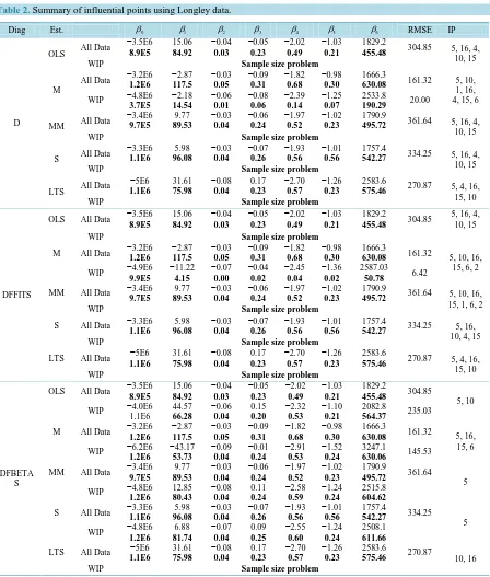
From Table 1, robust diagnostics based on OLS revealed that case 10 is an outlier. Robust diagnostics based on M estimator revealed that cases 10, 14, 15, 16 are outliers. Robust diagnostics based on MM and S estimators revealed that cases 14, 15, 16 are outliers while robust diagnostic measure based on LTS estimator revealed that cases 5, 14, 15, 16. The influential points from these outliers were then identified in Table 2. The robust diag-nostic measures identified more influential points than outliers; this might be because the Longley data suffers both multicollinearity and outlier problem.

(6)

[image:6.595.90.538.183.710.2]

Table 1. Summary of outlier results using Longley data.

Estimators Outliers

OLS 10

M 10, 14, 15, 16

MM 14, 15, 16

S 14, 15, 16

LTS 5, 14, 15, 16

Table 2.Summary of influential points using Longley data.

Diag Est. β0 β1 β2 β3 β4 β5 β6 RMSE IP

D

OLS All Data

−3.5E6 8.9E5 15.06 84.92 −0.04 0.03 −0.05 0.23 −2.02 0.49 −1.03 0.21 1829.2

455.48 304.85 5, 16, 4, 10, 15

WIP Sample size problem

M

All Data −3.2E6 1.2E6 −2.87 117.5 −0.03 0.05 −0.09 0.31 −1.82 0.68 −0.98 0.30 1666.3

630.08 161.32 5, 10, 1, 16, 4, 15, 6 WIP −4.8E6

3.7E5 −2.18 14.54 −0.06 0.01 −0.08 0.06 −2.39 0.14 −1.25 0.07 2533.8

190.29 20.00

MM All Data

−3.4E6 9.7E5 9.77 89.53 −0.03 0.04 −0.06 0.24 −1.97 0.52 −1.02 0.23 1790.9

495.72 361.64 5, 16, 4, 10, 15

S All Data

−3.3E6 1.1E6 5.98 96.08 −0.03 0.04 −0.07 0.26 −1.93 0.56 −1.01 0.56 1757.4

542.27 334.25 5, 16, 4, 10, 15

LTS All Data

−5E6 1.1E6 31.61 75.98 −0.08 0.04 0.17 0.23 −2.70 0.57 −1.26 0.23 2583.6

575.46 270.87 5, 4, 16, 15, 10

DFFITS

OLS All Data −3.5E6 8.9E5 15.06 84.92 −0.04 0.03 −0.05 0.23 −2.02 0.49 −1.03 0.21 1829.2 455.48 304.85

5, 16, 4, 10, 15

M All Data −3.2E6 1.2E6 −2.87 117.5 −0.03 0.05 −0.09 0.31 −1.82 0.68 −0.98 0.30 1666.3

630.08 161.32 5, 10, 16, 15, 6, 2 WIP −4.9E6

9.9E5 −11.22 4.15 −0.07 0.00 −0.04 0.02 −2.45 0.04 −1.36 0.02 2587.03

50.78 6.42

MM All Data −3.4E6 9.7E5 9.77 89.53 −0.03 0.04 −0.06 0.24 −1.97 0.52 −1.02 0.23 1790.9

495.72 361.64 5, 10, 16, 15, 1, 6, 2

S All Data −3.3E6 1.1E6 5.98 96.08 −0.03 0.04 −0.07 0.26 −1.93 0.56 −1.01 0.56 1757.4

542.27 334.25 5, 16, 10, 4, 15

LTS All Data −5E6 1.1E6 31.61 75.98 −0.08 0.04 0.17 0.23 −2.70 0.57 −1.26 0.23 2583.6

575.46 270.87 5, 4, 16, 15, 10

DFBETA S

OLS All Data −3.5E6 8.9E5 15.06 84.92 −0.04 0.03 −0.05 0.23 −2.02 0.49 −1.03 0.21 1829.2

455.48 304.85 _{5, 10}

WIP −4.0E6 1.1E6 44.57 66.28 −0.06 0.04 0.15 0.20 −2.32 0.53 −1.10 0.21 2082.8

564.37 235.03

M All Data −3.2E6 1.2E6 −2.87 117.5 −0.03 0.05 −0.09 0.31 −1.82 0.68 −0.98 0.30 1666.3

630.08 161.32 5, 16, 15, 6 WIP −6.2E6

1.2E6 −43.17 53.73 −0.09 0.04 −0.01 0.24 −2.91 0.53 −1.52 0.24 3247.1

630.06 145.53

MM All Data −3.4E6 9.7E5 9.77 89.53 −0.03 0.04 −0.06 0.24 −1.97 0.52 −1.02 0.23 1790.9

495.72 361.64 ₅

WIP −4.8E6 1.2E6 12.85 80.43 −0.08 0.04 0.11 0.24 −2.58 0.59 −1.24 0.24 2515.8 604.62

S All Data −3.3E6 1.1E6 5.98 96.08 −0.03 0.04 −0.07 0.26 −1.93 0.56 −1.01 0.56 1757.4

542.27 334.25 5 WIP −4.8E6

1.2E6 6.88 81.74 −0.07 0.04 0.09 0.25 −2.55 0.60 −1.24 0.24 2508.1 611.66

LTS All Data −5E6 1.1E6 31.61 75.98 −0.08 0.04 0.17 0.23 −2.70 0.57 −1.26 0.23 2583.6

575.46 270.87 10, 16

(7)

16, 4, 15 and 6 as influential. The points identified by Cook’s D based on MM, S and LTS estimators are not different from the points identified by OLS. Though with different root mean square error. The root mean square error is not too different.

The influential points identified by DFFITS based on OLS is not different from the cases identified using Cook’s D. Also, the cases identified by DFFITS based on S and LTS estimators respectively are not different from the points identified by their respective Cook’s D. The only exception is that DFFITS based on MM identi-fied more cases (5, 10, 16, 15, 1, 6, and 2) than its Cook’s D. The robust version of the DFFITS statistics based on the M estimator identified cases 5, 10, 16, 15, 1, 6 and 2 as influential.

From all the influential points identified by Cook’s D and DFFITS statistics respectively, the observations en-closed in parenthesis are reported to influence the regression coefficients. DFBETAS based on OLS (5, 10), DFBETAS based on M (5, 16, 15, 6), DFBETAS based on MM (5), DFBETAS based on S (5), DFBETAS based on LTS (10, 16). Cases identified by MM and S estimator are the same.

Having removed the influential cases, it can observed that the M estimator is most efficient (RMSED = 20.00,

RMSEDFFITS = 6.42, RMSEDFBETAS = 145.53). However, MM, S and LTS estimators could not provide results

probably because of small sample size (n = 16). More so, MM and S are modified M estimator.

[image:7.595.172.454.624.723.2]

3.2. Application to Scottish Hills Data

Table 3 and Table 4 provide the summary of results of the application of robust diagnostics measures to the Scottish Hills data.

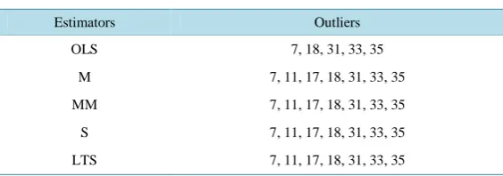
From Table 3, robust diagnostics based on OLS revealed that cases 7, 18, 31, 33, 35 are outliers. Robust di-agnostics based on the robust estimators (M, MM, LTS and S estimators) revealed that cases 7, 11, 17, 18, 31, 33, 35 are outliers. The influential points from these outliers were then identified inTable 4.

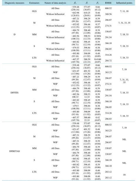
FromTable 4, Cook’s D based on OLS revealed that cases 7, 11, 18 (in this order) were the most influential cases. The robust version of the Cook’s D statistics based on the M estimator identified cases 7, 31, 33 and 35 as influential. The points identified by Cook’s D based on MM, S and LTS estimators are the same but with dif-ferent root mean square error.

DFFITS based on OLS revealed that cases 7, 18 (in this order) were the most influential cases. Case 11 iden-tified by Cook’s D was not ideniden-tified. Also, the cases ideniden-tified by DFFITS based on MM, S and LTS estima-tors respectively are the same with the cases identified by their respective Cook’s D.

From all the influential points identified by Cook’s D and DFFITS statistics respectively, DFBETAS based on OLS revealed that cases 7 and 18 affect the regression coefficients. The robust DFBETAS measures based on M, MM, S and LTS revealed that none of the influential points identified by DFFITS and Cook’s affect the regres-sion coefficients. It is concluded that the diagnostics measure computed using OLS is not reliable. For this data set, the diagnostic measures based on M estimator identified more influential points than other robust estimators. This might be because the RMSE is smaller than other considered estimators. However, MM, S and LTS esti-mators provided similar results.

Having removed the influential cases, it can observed that the M estimator is most efficient (RMSED = 274.31,

RMSEDFFITS = 274.31, RMSEDFBETAS = 286.87).

3.3. Application to Hussein Data

Table 5andTable 6provide the summary of results of the application of robust diagnostics measures to Hus-sein data.

Table 3. Summary of outlier results using Scottish Hills data.

Estimators Outliers

OLS 7, 18, 31, 33, 35

M 7, 11, 17, 18, 31, 33, 35

MM 7, 11, 17, 18, 31, 33, 35

S 7, 11, 17, 18, 31, 33, 35

(8)

[image:8.595.79.543.101.719.2]

Table 4. Summary of influential points using Scottish Hills data.

Diagnostic measures Estimators Nature of data analysis β0 β1 β2 RMSE Influential points

D

OLS

All Data −539.48 (258.16)

373.07 (36.07)

0.66

(0.12) 880.52

7, 11, 18 Without Influential −642.98

(128.83)

410.25 (28.01)

0.46

(0.09) 368.56

M

All Data −487.21 (89.26)

398.29 (12.47)

0.39

(0.04) 286.87

7, 31, 33, 35 Without Influential −452.02

(112.35)

396.46 (13.32)

0.37

(0.07) 274.31

MM

All Data −484.79 (97.50)

398.40 (12.09)

0.39

(0.06) 330.87

(100.33)

398.53 (12.33)

0.3854

(0.06) 291.54

S

All Data −483.82 (98.71)

398.45 (12.19)

0.39

(0.06) 366.10

(108.50)

398.84 (13.11)

0.38

(0.06) 286.85

LTS

All Data −493.80 _(93.16) _(11.92)398.09 _(0.05)0.40 314.26

(107.70)

388.59 (22.33)

0.4160

(0.07) 284.72

DFFITS

OLS All Data −539.48

(258.16)

373.07 (36.07)

0.66

(0.12) 880.52

7, 18

WIP −621.67

(113.86)

401.52 (15.26)

0.48

(0.06) 363.23

M All Data −487.21

(89.26)

398.29 (12.47)

0.39

(0.04) 286.87 7, 31, 33, 35

WIP −452.02

(112.35)

396.46 (13.32)

0.37

(0.07) 274.31

MM All Data −484.79

(97.50)

398.40 (12.09)

0.39

(0.06) 330.87

7, 18, 33

WIP −482.56

100.33

398.53 12.33

0.39

0.06 291.54

S All Data −483.82

(98.71)

398.45 (12.19)

0.39

(0.06) 366.10

7, 18, 33

WIP −479.5

(108.50)

398.84 (13.11)

0.38

(0.06) 286.85

LTS All Data −493.80 _(93.16) _(11.92)398.09 _(0.05)0.40 314.26

7, 18, 33

WIP −467.57

(107.70)

388.60 22.33

0.42

(0.07) 286.83

DFBETAS

OLS All Data −539.48 _(258.16) _(36.07)373.07 _(0.12)0.66 880.52

7, 18

WIP −621.67

(113.86)

401.52 (15.26)

0.48

(0.06) 363.23

M All Data −487.21

(89.26)

398.29 (12.47)

0.39

(0.04) 286.87

NIL

WIP −487.21

(89.26)

398.29 (12.47)

0.39

(0.04) 286.87

MM All Data −484.79

(97.50)

398.40 (12.09)

0.39

(0.06) 330.87

NIL

WIP −484.79

(97.50)

398.40 (12.09)

0.39

(0.06) 330.87

S All Data −483.82

(98.71)

398.45 (12.19)

0.39

(0.06) 366.10

NIL

WIP −483.82

(98.71)

398.45 (12.19)

0.39

(0.06) 366.10

LTS All Data −493.80

(93.16)

398.09 (11.92)

0.40

(0.05) 283.12

18

WIP −493.80

(93.16)

398.09 (11.92)

0.40

(9)

[image:9.595.89.540.230.718.2]

Table 5.Summary of outlier results using Hussein data.

Estimators Outliers

OLS 15, 16, 20, 21, 30, 31

M 12, 14, 15, 16, 17, 18, 19, 20, 21, 30, 31

MM 12, 13, 14, 15, 16, 17, 18, 19, 20, 21, 30, 31

S 12, 14, 15, 16, 17, 18, 19, 20, 21, 30, 31

LTS 12, 13, 14, 15, 16, 17, 18, 19, 20, 21, 30, 31

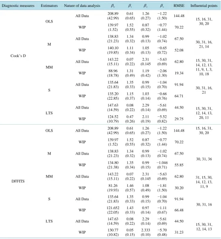
Table 6.Summary of influential points using Hussein data.

Diagnostic measures Estimators Nature of data analysis β0 β1 β2 β3 RMSE Influential points

Cook’s D

OLS

All Data 208.89 (42.99) 0.61 (0.65) 1.26 (0.27) −1.22

(1.50) 144.48 _{15, 16, 31,} 30, 20

WIP 139.97

(1.52) 1.52 (0.55) 0.87 (0.32) −0.77

(1.44) 70.22

M

All Data 138.83 (21.23) 1.34 (0.32) 0.99 (0.13) −1.02

(0.74) 67.50 _{30, 31, 16,} 21, 14

WIP 140.10

(19.85) 1.11 (0.34) 1.05 (0.13) −0.65

(0.72) 52.08

MM

All Data 143.22 (15.11) 0.07 (0.22) 2.31 (0.145 −5.63

(0.69) 62.80 15, 30, 31, _{14, 12, 13,} 11, 9, 1, 3, 10, 18

WIP 88.96

(18.78) 1.31 (0.49) 1.19 (0.42) −2.06

(1.30) 19.34

S

All Data 135.64 (21.83) 1.35 (0.33) 0.99 (0.15) −1.04

(0.70) 91.94 _{30, 31, 16,} 21

WIP 135.20

(22.85) 1.15 (0.37) 1.03 (0.14) −0.66

(0.76) 64.71

LTS

All Data 147.63 (14.59) 0.08 (0.22) 2.29 (0.14) −5.61

(0.69) 44.50 15, 30, 31, 12, 14, 13, 20, 11

WIP 124.52

(10.79) 0.47 (0.26) 2.11 (0.19) −5.52

(0.82) 29.75

DFFITS

OLS All Data _(42.99)208.89 _(0.65)0.61 _(0.27)1.26 _(1.50)−1.22 144.48 15, 16, 31, _{30, 20}

WIP 139.97

(1.52) 1.52 (0.55) 0.87 (0.32) −0.77

(1.44) 70.22

M All Data 138.83

(21.23) 1.34 (0.32) 0.99 (0.13) −1.02

(0.74) 67.50

30, 31, 36

WIP 134.80

(21.38) 1.35 (0.34) 0.99 (0.15) −1.046 (0.71) 55.85

MM All Data 143.22

(15.11) 0.07 (0.22) 2.31 (0.145 −5.63

(0.69) 62.80 31, 15, 30, 14, 12, 13,

11, 9

WIP 81.26

(19.93) 1.46 (0.57) 1.08 (0.49) −1.81

(1.50) 30.20

S All Data 135.64

(21.83) 1.35 (0.33) 0.99 (0.15) −1.04

(0.70) 91.94

30, 31, 16

WIP 121.652

(22.05) 1.43 (0.33) 0.97 (0.14) −1.11

(0.67) 66.48

LTS All Data 147.63

(14.59) 0.08 (0.22) 2.29 (0.14) −5.61

(0.69) 44.50 _{15, 30, 31,} 12, 14, 13

WIP 130.77

(10)

Continued

DFBETAS

OLS All Data 208.89 (42.99)

0.61 (0.65)

1.26 (0.27)

−1.22

(1.50) 144.48

15, 16 WIP 181.85

(45.22)

1.52 (0.86)

0.65 (0.60)

−0.00

(2.27) 134.01

M All Data 138.83 (21.23)

1.34 (0.32)

0.99 (0.134)

−1.02

(0.74) 67.50

NIL WIP 138.83

(21.23)

1.34 (0.32)

0.99 (0.134)

−1.02

(0.74) 67.50

MM All Data 143.22 (15.11)

0.07 (0.22)

2.31 (0.145

−5.63

(0.69) 62.80

NIL WIP 143.22

(15.11)

0.07 (0.22)

2.31 (0.145

−5.63

(0.69) 62.80

S All Data 135.64 (21.83)

1.35 (0.33)

0.99 (0.15)

−1.04

(0.70) 91.94

NIL WIP 135.64

(21.83)

1.35 (0.33)

0.99 (0.15)

−1.04

(0.70) 91.94

LTS All Data 147.63 (14.59)

0.08 (0.22)

2.29 (0.14)

−5.61

(0.69) 44.50

NIL WIP 147.63

(14.59)

0.08 (0.22)

2.29 (0.14)

−5.61

(0.69) 44.50

From Table 5, robust diagnostics based on OLS revealed that cases 15, 16, 20, 21, 30, 31 are outliers. Robust diagnostics based on M and S estimators revealed that cases 12, 14, 15, 16, 17, 18, 19, 20, 21, 30, 31 are outliers. Robust diagnostics based on MM and LTS estimators revealed that cases 12, 13, 14, 15, 16, 17, 18, 19, 20, 21, 30, 31 are outliers. The influential points from these outliers were then identified inTable 6.

From Table 6, Cook’s D based on OLS revealed that cases 15, 16, 31, 30, and 20 (in this order) were the most influential cases. The robust version of the Cook’s D statistics based on the M estimator identified cases 30, 31, 16, 21 and 14 as influential. The robust version of the Cook’s D statistics based on the MM estimator identified cases 15, 30, 31, 14, 12, 13, 11, 9, 1, 3, 10 and 18 as influential. The robust version of the Cook’s D statistics based on the S estimator identified cases 30, 31, 16 and 21. The robust version of the Cook’s D statistics based on the LTS estimator identified cases 15, 30, 31, 12, 14, 13, 20 and 11 as influential.

The cases identified by DFFITS based on OLS is not different from the ones identified using Cook’s D. The cases identified by DFFITS based on M and S estimators are 30, 31 and 36. The robust version of the DFFITS statistics based on the MM estimator identified cases 31, 15, 30, 14, 12, 13, 11 and 9 as influential. The robust version of the DFFITS statistics based on LTS estimator identified cases 15, 30, 31, 12, 14 and 13 as influential.

From all the influential points identified by Cook’s D and DFFITS statistics respectively, DFBETAS based on OLS revealed that cases 15 and 16 affect the regression coefficients. The robust DFBETAS measures based on M, MM, S and LTS revealed that none of the influential points identified by DFFITS and Cook’s affected the regression coefficients.

It is concluded that the diagnostics measure computed using OLS is not reliable. For this data set, the diag-nostic measures based on MM estimator identified more influential points than other robust estimators. This might be because the RMSE is smaller than other considered estimators.

4. Conclusions

(11)

that root mean square error value reduces as the influential points are identified and removed. The DFBETAS shows that not all cases reported to be influential exert undue influence on the regression coefficients. The di-agnostic measures based on the robust estimators perform better than OLS estimator when the influential points are removed or not. Also, the performance of the proposed robust diagnostics measure based on MM performs better than that of M estimator in application to Hussein data.

Finally, the performances of the proposed robust diagnostics measured based on MM and M estimator are generally more efficient based on the applied data.

References

[1] Barnett, V. and Lewis, T. (1994) Outliers in Statistical Data. New York, Wiley.

[2] Belsley, D.A., Kuh, E. and Welsch, R.E. (1980) Regression Diagnostics; Identifying Influence Data and Source of Col-linearity. Wiley, New York. http://dx.doi.org/10.1002/0471725153

[3] Chatterjee, S. and Hadi, A.S. (1988) Sensitivity Analysis in Linear Regression. Wiley Series in Probability and Ma-thematical Statistics. Wiley, New York. http://dx.doi.org/10.1002/9780470316764

[4] Turkan, S., Meral, C.C. and Oniz, T. (2012) Outlier Detection by Regression Diagnostics Based on Robust Parameter Estimates. Hacettepe Journal of Mathematics and Statistics, 41, 147-155.

[5] Chen, C. (2002) Robust Regression and Outlier Detection with the ROBUSTREG Procedure. Proceedings of the Twenty-Seventh Annual SAS Users Group International Conference, SAS Institute Inc., Cary, NC.

[6] Gujarati, N.D. (2003) Basic Econometrics. 4th Edition, Tata McGraw-Hill, New Delhi, 748, 807

[7] Huber, P.J. (1973) Robust Regression: Asymptotics, Conjectures and Monte Carlo.Annals of Statistics, 1, 799-821. http://dx.doi.org/10.1214/aos/1176342503

[8] Rousseeuw, P.J. and Yohai, V. (1984) Robust Regression by Means of S Estimators in Robust and Nonlinear Time Se-ries Analysis. In: Franke, J., Härdle, W. and Martin, R.D., Eds., Lecture Notes in Statistics, 26, Springer-Verlag, New York, 256-274.

[9] Rousseeuw, P.J. and Leroy, A.M. (1987) Robust Regression and Outlier Detection. Wiley Interscience, New York (Se-ries in AppliedProbability and Statistics), 329 pages. http://dx.doi.org/10.1002/0471725382

[10] Yohai, V.J. (1987) High Breakdown Point and High Efficiency Robust Estimates for Regression. Annals of Statistics,

15, 642-656. http://dx.doi.org/10.1214/aos/1176350366

[11] Rousseeuw, P.J. and van Driessen, K. (2006). Computing LTS Regression for Large Data Sets. Data Mining and Knowledge Discovery, 12, 29-45. http://dx.doi.org/10.1007/s10618-005-0024-4

[12] Cook, R.D. (1977) Detection of Influential Observations in Linear Regression. Technometrics, 19, 15-18. http://dx.doi.org/10.2307/1268249