The transfer of statistical equilibrium from physics to economics

(1)

The transfer of statistical equilibrium

from physics to economics

Parrinello, Sergio and Fujimoto, Takao

Università di Roma "La Sapienza", Okayama University

1995

Online at

https://mpra.ub.uni-muenchen.de/30830/

(2)

THE TRANSFER OF STATISTICAL EQUILIBRIUM

FROM PHYSICS TO ECONOMICS

Sergio Parrinello (University of Rome “La Sapienza")

and Takao Fujimoto (Okayama University)

1995

(3)

ABSTMCT

Two

applications

of

the

concept

of

statistical

equilibrium, taken

from

statistical

mechanics, are compared: a simple model

of

a pure exchange economy, constructed as

an alternative to a walrasian exchange equilibrium,

and

a simple model

of

an industry,

in which

statistical

equilibrium is

used as

a

complement

to

the

classical

long

period

equilibrium.

The postulate

of

equal

probability

of

all

possible microstates

is

critically

re-examined. Equal probabilities are deduced as a steady state

of

linear and non-linear

(4)

2

Introduction

The

concept

of

statistical

equilibrium

is a

fundamental

analytical

tool

in

physics and

particularly

in

statistical mechanics.

After

having borrowed

the

classical

mechanics concept

of

equilibrium,

economic

theory has

occasionally

turned

its

attention

to

the

other

concept

of

probabilistic equilibrium.

In

fact,

since

the

contributions

which

appeared

in

the

50s and

the

early 60s

it

is

only

recently

that

serious

attempts

have

been

made

to

revise

and

develop

the notion

of

statistical

equilibrium

in

economics. Past contributions

include

Champernown

(1953),

Simon-Bonini

(1958),

Newman-Wolf

(1961) and Steindl (1962) and were

mainly

related to

Gibrat's Law

(1931)

and

to

Pareto

distribution.

Recent

works,

explicitly linked

to thermodynamics, are

E. Farjoun

-

M.

Machover

(1983)

and, in paficular,

Foley (1991, 1994) .

In

economics a statistical

equilibrium is

a most probable distribution

of

certain economic entities (say firms or individuals) which cannot all be distinguished one

from

another, rather

than a particular configuration

in

which

each

entity is

identified.

In

other words,

this

equilibrium

is

a

macrostate

with

maximum number

of

realizations

(microstates) and, as such,

is

a distinct

concept

from

a

state obtained

by

the

simple

inclusion

of

some random

variable

in

the

relations

which

determine

a

classical

equilibrium.l

In

this

work two

applications of the concept

of

statistical

equilibrium

to

economic theory

will

be formulated and compared using simple models. Furthermore

it

will

be

shown

that, under sufftcient

conditions,

a

state

of

equal

probability

of

microstates - a basic postulate

in

statistical mechanics

-

in the long period is consistent

with

unequal transition probabilities.

In

section

1 the

first

application

is

a

model

of

a

pure

exchange economy, constructed as a special case

of

Foley's (1994) model

in

which

statistical

equilibrium

appears

as an

altemative

to

the

Walrasian

equilibrium.

In

section

2 the

second

application

is

a

model

of

an industry

in

which

statistical

equilibrium

is

used

as

a

complement

to

the

classical

long

period

equilibrium.

It will

be

argued

that

only

the

latter application maintains the notion

of

statistical

equilibrium

adopted

in

the

field

of

physics; whereas the former differs from

it

on an essential point and resolves

itself

into

a

concept

of

equilibrium

similar

to

that

of

temporary

equilibrium

adopted

in

economics.

In

section

3 the

postulate

of

equal

probability

is re-examined

and

a simple case of linear Markov chains is presented, in which equal

probability

is a steady

state

of

a

stochastic

process.

In

section

4 this

uniform probability

outcome is generalized

to

non-linear

Markov

chains, applying a theorem proved

by Fujimoto

and Krause (1985).

(5)

Let

us

make

a

simple

example

of

statistical

equilibrium

for

an

exchange

economy, as

a

special case

of the

statistical

theory

of

markets developed

by

Foley

(1991-1994). In this theory the elementary unit of analysis is the

individual offer

set :

"The marlret

begins

with

agents

defined

by offer

sets

reflecting

their

information,

technical pos sibilitie s, endowments and preferenc e s " (p. 3 2

4. "In

terms

of

standard production-exchange model,...., offer sets consist

of

technically

feasible

transactions leading to

_Jìnal

consumption bundles that are

preferred to

initial

endowments" ( Foley p.32a)

Suppose

that

there are

only

4

agents

e,o2,bt,b2

and

two

goods

X,Y

the

quantities

of which

are measured

by

integers. There is a total

of

4 units

of

good

X

and

4 of

good

Y

which

are equally distributed at the beginning: each

individual

therefore has an endowment of one unit of each good. V/e

will

athibute to the agents very simple preferences: agerrts

ar,a.,

like

good

X,

but

are

indifferent

to

good

Y;

whilst

agents

br,b, like

good

Y,

but

are

indifferent

to

good

X. An

agent's transaction

is

a vector

of

quantities

of

the

two

goods

with

a plus sign

to

indicate a net acquisition, a minus sign

for

a net cession and zero

if

the

initial

endowment is maintained.

The

offer

set

of

an agent is the set of transactions

which

are

weakly

preferable

to and feasible for

him

in relation to his

initial

endowment. In Foley's model the

agents

that

have

the

same

offer

set are considered indistinguishable and represent a

tvoe

of

asent.

In the figures below the lattices represent parts

ofthe

offer sets ofagents

oftype

A

and

B

as

feasible transaction

sets.

The

null

transaction

(0,0)

is

included among

the

(6)

Type A

2

Type B

In

the

example

we

can therefore

find two

types

of

agents:

type

A

(to which

ar,a,

belong) and type

B

(to which

br,brbelong).

These types can be identified by their

offer

sets

which

are

distinct

as

far

as

their

preferences are concemed,

but not

for

their

endowments.

Table

I

describes the feasible microstates of the exchange economy.

TABLE.

I

(0 0)

(r

-1) (-1

l)

ar _ra,_,br_rb,

ar _rb qr b,

Ar,b. a1 b1

a"b, al b.,

arb, ar b1

0t ,Cl, br,b,

It

is

to

be noted that no exchange takes place

in

the

first

microstate and each agent

in

the last one acquires one

unit

of

his preferred good against one

unit

of

his indifferent

good.

In

the other

four

microstates

two

agents make one preferred transaction,

whilst

the other

two

remain in their

initial

position.

Let us

consider

the

feasible

statistical

aggregates

or

macrostates

of

the

exchange

economy

by

treating

agents

of

the

same

type as

indistinguishable

and

[image:6.604.65.523.60.290.2]

(7)

we

find

three macrostates,

two

of which are made

of

only one microstate (the

first

and the last one represented in table

I)

and one made by four microstates (the others).

Let us assign equal probabilities to all feasible microstates.

A

statistical

equilibrium

is

a macrostate

with

maximum

probability, that

is with

the

maximum number

of

feasible equally

probable

microstates.

In

the

example this

macrostate is the one

with

four microstates, in which, for each type

of

agent, one of the

two

benefits from the exchange by acquiring a

unit

of his preferred good and

by giving

up a

unit

of the indifferent good, whilst the other agent remains at the status quo.

A

market statistical equilibrium in the model developed by Foley possesses the

following

interesting features

that

contrast

with

those shared

by

a

walrasian general

equilibrium:

1.In general

it

is not Pareto-efficient;

2.It

does

not

imply

a

uniform

exchange ratio between

each

pair

of

commodities over

all

transactions;

3.A uniform

entropy price

is

associated

to

each

good:

this

price

is

a shadow price

determined

by

solving

an entropy

maximizing

problem under the

total

endowment constraints.

Property

I

is

straightforward

in

our exchange model, as the most probable macrostate

is Pareto-inferior compared to that in which all the agents obtain a

unit

of the preferred good

in

exchange

for

the other good. Instead properties

2

and 3 are not evident

in

this simple model and

we

shall

not

be concerned

with

them

for

the sake

of

the

following

argument.

It

should

be

emphasized

that

the

statistical

equilibrium

of

the

exchange

economy

is

determined

by offer

sets

that

depend

on the

initial

endowments

of

each

individual.

In

general

the

offer

sets undergo endogenous change

if

the

economy is conceived

in

real time. To make this point clear,

it

is

suffrcient

to

assume that the

two

goods are

non

perishable

and

that the

economy

is

subject

to

two

trials

and two

corresponding observations. Let us suppose that the

following

microstate is realized

in

the

first trial:

Then at the second

trial

the individual endowment

will

differ

from that at the beginning

of

the

first

trial.

Therefore the types

of

agents and the number

of

each type

will

differ

(8)

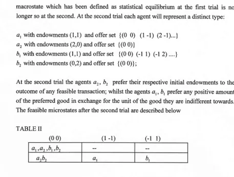
macrostate

which

has been

defined

as statistical

equilibrium

at the first

trial

is

longer so at the second.

At

the second

trial

each agent

will

represent a distinct type:

a, with

endowments

(1,1)

and offer

set

_{(0

0)

(l

-l)

(2 -l)...\

a,

with

endowments (2,0) and offer

prefer

their

respective

initial

endowments

to

the outcome of any feasible transaction; whilst the agents ar,

b,

prefer any positive amount

of the preferred good

in

exchange

for

the

unit

of the good they are indifferent towards. The feasible microstates after the second

trial

are described below

TABLE

II

(0 0)

(l

-l)

(-l

1)

ar _ro,_,br_rb,

o"bt qr _bl

From the statistical

point

of

view

the sample space has changed. The

two

microstates

in table

II

each have

probability

ll2

at each

trial.

Howevef, as the trials are repeated an

indefinite

number

of

times,

the

second microstate

will

be

realized

with probability I

and

when

that

happens

the

economy

will

have

reached

a

Pareto-efficient configuration.2

At

that point the

of[er

set

of

each agent

will

be represented by the

null

vector (0,0), that is by the absence of any further transaction.

One

may

well

ask whether

the

statistical

equilibrium

of

exchange, as defined above, preserves

the

concept

of

statistical

equilibrium

in

physics.

The

answer

is

no.

The latter has the relative persistence

of

its determinants

in

common

with

the classical

equilibrium

in

economics;

by

contrast,

the

statistical

exchange

equilibrium,

as

illustrated

in

the

example, does

not

possess

this

prerequisite and

from this point

time,

it

becomes

a

model

of

statistical disequilibrium,

with

certain

transition

probabilities

that

imply an

absorbing

microstate.

This

state

is a

Pareto-efficient

2In _a_certain_sense_the_agenl.s_ar,a2,b1,b,_cottld_not_be_{distinguished}_{into type}_A_and_B_{right from the very}_first

trial if "distinguishability" also requires "observability". In fact at the beginning all agents have the same initial

[image:8.612.75.532.66.411.2]

(9)

equilibrium.

The stochastic

feature

is

inherent

only

in

the adjustment

(or

relaxation)

process but not

in

the

final equilibrium

of the exchange.

In

a more general model

with

many Pareto-effrcient microstates, we

would

find

a problem

of

indeterminacy

similar

to

the

one

found

in

a Walrasian exchange

model

if

we

assume that transactions can

occur at

disequilibrium

prices

in

the

adjustment process towards

equilibrium.

In

this

endowments.

As

a

consequence,

the

statistical exchange

equilibrium

with

a microstate which takes

probability

I

at the

limit.

2.

A

model of stotisticol eauilibrium of the industrv

Now we

shift

to

a more

poúe

application

of

statistical

equilibrium.

Let

us suppose

now that an

industry

is

in

a

long period

competitive

equilibrium,

under constant retums to scale at the

firm

level. Suppose that its product can take

only

integer numbers 1,2,3,...

Let

_{Q be the}quantity produced and

N

the number of firms

which

can

produce at

the minimum

cost per

unit of

output.

With

these hypotheses,

if

D

is

the demand

for

the product at

the long

period prices, the theory

of

classical

equilibrium

determines Q from the equation

Q:

D, but does not determine the size of each

firm.

Let us

consider

now the

feasible microstates

of

the industy which

can

be obtained

by

distributing

in

every possible

way

the

N

firms

among the possible sizes measured

by the

quantities 0,1,2,3....

In

order

to

illustrate

this we

will

present an example similar to that used by

others (A.

F.

Brown,

1967) to introduce the concept

of

statistical

equilibrium

with

reference

to

the

distribution

of

a given

amount

of

energy among

agivennumberof

particles of aperfect gas.

Letus

assume

Q:3;

N:4

and

(10)

I

TABLE

III

Firm

size measured by amounts of output

t2

1l (a) (b) (c) (d)

2l (a)

(b)

(d) (c)

3l

(a)

(c)

(d) (b)

4l

(b)

(c)

(d) (a)

sl (a) (b) (c) (d) 6l (a) (b) (d) (c)

71(a)

(c) (b) (d)

8l

(a)

(c) (d) (b) el

(a)

(d) (b) (c)

101

(a)

(d) (c)

o)

l

ll

_G)

(c) (a) (d)

I2l

(b)

(c) (d) (a)

131 (b)

(d) (a) (c)

r4l

o)

(d) (c) (a)

151 (c)

(d) (a) (b)

161 (c)

(d) (b) (a)

t7l

(a)

(b)

(c)

(d)

181 _O)

(a) (c)

(d)

lel

(c)

(a)

(b)

(d)

201

(d)

(a)

(b)

(c)

Let

us

adopt

the term

"macrostate"

to

indicate

a

statistical

aggregate

of

microstates (a distribution), obtained by assuming that the firms are not distinguishable

from

each other. The firms are not distinguished either because we are not interested

in

their identification

or

because

they

cannot

be

distinguished.

In

our

example three macrostates of the industry are feasible

- three inactive

firms

and a

firm of

size 3;

J

[image:10.612.57.578.71.774.2]

(11)

-

two

inactive

firms,

a

size-l firm

and

asize-2frmr;

- one inactive

firm

and three

size-l

firms.

The

first

macrostate

is

generated

by

the

hrst four

microstates; the second

by

the next

12 and the

third

by the last four.

In the general case let us indicate

n:

(no,n1,/t2,....,ne)

a feasible macrostate

in

which

no

firms

are size

0, n, firms

are size

|,....,no

firms

are size _{Q on the}condition that

no+ntnr....nn=N

(l)

Let w(n) be the

number

of

feasible

microstates

with

distribution

n :

(no,nr _{rÍ12,....rflg).}

Combinatorial analysis gives

rr(n)= . .t'.

,

nolnrlnr!...nn1,

where by convention

0!:1.

(2)

A

macrostate

n:

(n0,nr,fi2,....,flg)

is

feasible

if

it

satisfies, besides the

equality

(l),

the conservation condition of the total quantity _Q

Ùno

+ln,

+2n,

+'..+

_Qro

₌

Q

(3)

The total number of feasible microstates is

z

=

lw(n),

with

summation over all macrostut",

whiclisatisfr

(1) and(3).

We may have an idea of the order of change in

w(n)

in response to variations

in

n,

as the number

of firms

is

slightly

larger than the number represented

in

the table,

if

we assume3

N:

20

and

Q:20.

In this case, we

will

have for the macrostate made up

of

8 inactive

firms, 6

size-l frrms, 4 size-2

firms

and

2

size-3 firms:

201

w =

-

=2x108.

8t6l4t2l

By

contrast for the macrostate in which all the firms are of a

uniform

size equal

to

I

we

find

201

w- '-1.

201

It

is clear how enormous the difference is between the

multiplicity

of microstates in the

first

case,

which

represents

a

decreasing

distribution

compared

with the

single

(12)

10

microstate

with a

uniform distribution. So

far we

have

followed

combinatorial

analysis.

To move onto the

concept

of

statistical

equilibrium we

have

to

assume a

probability

distribution.

In

statistical physics

we find

more

than

one assumption

of

probability on this point.

In

the so-called Maxwell-Boltznann distribution

equal

probability is

athibuted to each microstate; different assumptions

of probability

can be

found, however, at the basis of the Bose-Einstein and of the Fermi-Dirac distributions.a

V/e

will

adopt the Maxwell-Boltzmann hypothesis

of

equiprobability

initially

as an a

priori;

then we

will

obtain this uniform probability from other assumptions.

In

the

example illustrated

in

table

III,

each microstate has

probability

1/20;

whilst

the three macrostates have respectively probabilities

l/5, 315,ll5.

The statistical

equilibrium

of

the industry

is

the second macrostate

with

probability

3l5.In

this

case

the small number

of

microstates, used

for

the purpose

of

the exposition, does

not

yet

enable

us

to

attribute a useful theoretical role

be solved

maxr.r,(n)

=

noftt*-"ne

nolnrlnrl...nnl

subject

to

no + nt

t

n2r....nn

=

N

Ùno

+ln,

+2nr+...+Qnn

:

_Q.

By

adopting a

similar

demonstration to that given

in

statistical physicss, the

following

solution,

as

shown

in

Appendix

I,

can

be

obtained

by

an

approximation

in

the

continuum and for

N

_{and Q large numbers.}

N!

e-pt

4 = ^i o

I

s =

o,1,...,e.

S

tv

_--F"

L/

s=0

(4)

with

_{p =}

l^(I

+

where

ln

is the natural logarithm.

;)

>

0. (s)

4 _For_a_{comparison of}_{Maxwell-Boltanann's,}_{Bose-Einstein's and}_{Fermi-Dirac's}_{so-called statistics,}_see

W. Feller (1970).

(13)

Hence

the

most

probable

macrostate

n

is

a

distribution

of

_firms

which

decreases

according to a geometric progression as the size increases; as

no nl

_{...,....nr_,}

=

_",

.

(6)

nt

n2 ne

From (5) we obtain

eF

-r

Having reached

this

result, the

initial

assumption that _Q,the quantity produced

by

the

industry,

is a

quantity

in

non-statistical classical

equilibrium,

determindd

on

the demand side, becomes important. Substituting

Q:

D in

(7), we obtain:

eF

-l

Equations

(6)

and

(8)

show

that

as

the

demand

D

increases,

ceteris

paribus,

the coeffrcient

p

decreases and, therefore,

the

dispersion

of firms

among classes

of

ever

increasing size grows.

It

is worth noting

that the

ratio

DA.{,

demand per number

of

ftrms, plays

a

similar role

to

that

played

by

temperature

T

in

the

corresponding

physical problem determining the most probable

distribution

of

particles

or

harmonic oscillators among a certain amount of energy.

Entroplt

We can interpret the

equilibrium

of the industry

in

terms

of

entropy.

Let

p,

be the

probability

of

microstate

i;

and let us measure the improbabilify

of

microstate

i

by

the logarithm

010

J-XI,

---LrLp..

_P,

t

We can then define entropy

S(n)

of ttre macrostate n the average

improbability of

the microstates of which

it

is composed, where the weights are the probabilities

p,:

O_

N

(8).

D

N

(7)

w(n)

S(n)

: -I

L

(14)

1,2

If

all

microstates

in

the macrostate

n

have

probability

p,

nis

the entropy

of

S(n)

=

!^*6)

and

the

entropy

of

a

most

probable

macrostate

n is S(n) = I*

_w

_(n).

Therefore

s

statistical equilibrium of

the industry

is

a

macrostate

that

has maximum entropy; hence, under the assumption of equal probability, a macrostate

with

maximum

h/(n)

number

of

possible realizations.

As

N

increases,

the

ratio

_;

decreases,

whilst

t)

lxù

rnl(n)

----n-

tends

to

1, where m

is

the total number

of

microstates. Then,

for

N

large,

Lnm

the

entropy

of

the

industry

in

its

most

probable

state

can

be

written

n

S(w(n)

) = lnn.

_Since

_the

_{improbability}

_of.

a

_macrostate

n

is

0m0n

LrL-

- Ln m-dn

w(n),

we

can

also

say

that

for

a

large

N

a

statistical

w(n)

equilibrium belongs to a set of macrostates

with

almost zero

improbability,

in the sense

that

w(n)turns

out

incomparably greater

than

w(n)

associated

with

any

other

macrostate n outside the equilibrium set.

This property means that a macroscopic regularity

(equilibrium)

exists

in

terms

of

firm

distribution.

Such

regularity

emerges

in

real

time,

if

we

suppose

that

the number of

potential

firms

N

and the quantity

in

demand

D

are stationary.

A

statistical

equilibrium

can therefore be considered

other scenes: when the

film

is run

at a

sufficiently high

speed,

the viewer

is

hardly

aware

of

these

odd

scenes

at

all, whilst

he perceives

does

presuppose

it

and

stands

as

a complement

to it. In

fact the stationarity

of

_{Q is not}

a physical necessity

(like

energy conservation), but rather a property

of

classical

equilibrium

in

which

_Q

is

determined

by

the

effective

demand at the

long run

competitive prices.

It

is

to

be noted that the

stationarity of the most probable distribution of firms hides an incessant movement at a

microeconomic level:

if

it

were possible to observe the trajectory of each

firm

(a not so

be true

in principle.

In

economics, as

in

the physics

of

gas, the number

of

units involved has

to

be

large

for

this

concept

to

be

of

use

for

the analysis. Thus

in

the model

of

the industry

the number

of

firms

N

has to be large enough.It must be noted, incidentally, that there

are some

diffrculties

in

observing

N,

in

so

far

as many

potentially active

firms

are

inactive

in

equilibrium. Also

the quantity _Q,

which

is measured

by

integers, had

to

be assumed

to

be large

for

the pu{pose

of

the

solution

given

in

appendix

I. Clearly

the

analysis

and then

equal

probability

is

assigned

to

these microstates. This analytical level is chosen on the basis of the

logic

of the problem,

of

a separate theory or

of

an

intuition,

the usefulness of this choice being tested by its predictive capability.

In

applying the statistical

equilibrium

approach,

two

methodological

pitfalls

should be

avoided.

With

respect to the phenomenon under investigation: a) the assumed sample space

might

lack

persistency and

b)

the

assumed microstates

might not

have equal

probability.

Let

us

examine

now

the

applications

of

the

statistical equilibrium

approach

to

the

exchange economy (section

1)

and

to

the

economy

of the

industry

(section

2)

atthe

light

of the above criterion.

In

the

application

to

the

exchange economy,

the

choice

of

behaviour.s

In

this

case

it

is

hard

to

explain

why

the

probability

of

a

Pareto-effrcient microstate

is

and remains

not

greater

than

the

(16)

L4

probability

first

row

of

Table

I

does not

represent any Pareto-improvement,

but

it

has, nevertheless, been athibuted

the

same

probability

as any

of

the other microstates (described

in

the other rows) that do

in

fact

imply

an

improvement. We

observe

that the latter

problem prevents

the

exchange

statistical

equilibrium from

strengthening

its

theoretical

role

initial

endowments does

not arise.

In

the pure exchange economy let us assume the goods to be labour services, instead

of

durable goods, and the

initial

endowments to be made up

only of

persistent

labour capacities

of

workers to provide those services.

By

this hypothesis,

if

we assign

all

the

feasible microstates equal

probability,

it

is

possible

to

formulate

a

statistical

equilibrium

for

the

exchange

of

labour services

in

real

time,

instead

of

a temporary statistical

equilibrium.

In

spite

of

this,

there

still

remain

the

same objections

to

the

hypothesis

of

equal

probability:

as

if

on each

trial

the agents described

by

the model

would

look

for

each other and accept

with

equal chance any transaction which does not

entail

an inferior position

for

them,

compared

to

the

absence

of

exchange. The

rationality

of these agents seem to be minimal.

It

would be more reasonable to attribute

equal

probability

to

those

microstates

which

imply

Pareto-efficient allocations

of

labour-services and lower probabilities

hand,

we observe that the choice

of

the sample space, made

of

all

possible microstates of the industry, belongs to

the

general model of placing randomly

a

given

number

of

balls

(firms)

in a

given

number

of

cells

(firm

sizes);

then aggregation runs by treating the balls as indistinguishable, whereas the cells are kept as

distinct

entities.

I

This

model

might not

be appropriate,

if

the distribution

of

many

customers among

many

firms

is

an essential

element

in

the

enumeration

of

the microstates

of

a production system

with

exchange.

Suppose

for

simplicity

that

in

the

model

described

by

Table

III

there are three customers and each customer demands

one

unit

of

outptut,

as

if he

would

represent an economic "quantum".

In this

case,

7 _Foley_himself_in_his_working_paper_(Foley,_l99l)_assumed_as_feasible_only_{those microstates}_which

imply Pareto-superior and efficient allocations.

(17)

many microstates

listed

in

table

III

must be re-interpreted

as

composed events:

for

instance

row

1

would

stiill

describe

a simple event

with

a single realization,

in

which

firm

(d)

supplies one

unit

of

output

to

each customer, whereas

the other

firms

(a),(b),(c) are

inactive;

by

contrast

row

5 would

describe a composed

event

with

3

rcalizations, as

firm

(c)

can supply one

residrlal

customers

and

firms (a),

(b)

remain

inactive.

From

this

perspective,

many microstates

in

Table

III

should be conceived as macrostates that must be decomposed

in

further

microstates

by

replacing

the occupancy

model

of

balls

and cells

with

a

model

that

counts

all

possible

ways

for

assigning

three

quanta, initially

distinguishable,

to

four

particles,

initially

distinguishable

as

well.

Only at

this

extended

micro-level, the

equal

probability

assumption should

be applied

and the

definition

of the macrostates should be chosen.

On the

other

hand,

the

equal

probability

assumption

refers

to

absolute

probabilities.

It

remains

to

be proved that a state

of

uniform

absolute

probability is

a steady state outcome

of

a stochastic process and that this outcome is independent

from

the

initial

probability

vector.

In

particular,

in

period

of

time.

Thus,

in

the

example described

in

Table

III, it

can

be supposed that,

if

the

initial

microstate is the one described

in line

I

(with

flrms

a,b,c,

inactive and

firm

d

of

size 3),

it

can be more probable that microstate 5

(with

firms

a

and

b

still

inactive,

f,rrm

c

af

size

I

and

firm

d

at

síze

2)

will

be

realized

in

the

following trial

than microstate

2 (firms

a,b,d inactive and

firm

c

of

size 3). However,

under certain assumptions, these unequal conditional probabilities are compatible

with

equal

absolute

probability

of

all

possible

microstates.

In

particular

it

can

be

immediately proveds, using the theory

of Markov

chains that,

if

the

transition

matrix

is

given and

it

is

a

doublv

stochastic and

primitive,lo

then

all

microstates take equal

probabilities

at

the

limit

of

a

series

of

repeated

trials

and

this uniform probability

is

independent

of

the

initial

microstate

(or,

more

generally,

of

the

initial

probability

vector).

A

special case

of

doubly

stochastic transition

matrix

arises

if

we

assume that

reversibility

exists

in

the

probabilistic

sense between each

pair

of

microstates

of

the

e _See_{Feller (1970),}_chapter_XV_page_399;_{and Seneta}_(1973). 10

Let

pii

be the transition probability from microstate i to microstate

i

in one trial and let

"

= t;l1) the mxm

(18)

L6

industry at each

trial;

that is the

probability

that the microstate

i

occurs,

following

the

realizatíonof

the microstate

j,

is the same as the probability that

j

occurs,

following

the

realization

of

i.

This

hypothesis

is

represented

by

a

mxm

symmetrical transition matrix.

In

the

it

will

be proved that equal probabilities can be deduced as

a

limit

property under assumptions less restrictive than that of double stochasticity.

4.

Equal

probabílity through

non-línear

Markov

chains

with

lagged variables.

Let us introduce time

lags

and

write

xr*l

= f

(x,

_,xr-,

,....rxt-^)

for

t

= 0r1r2,....

The

vector

x,

₌

(r,r ,xp1...exs,)'

shows the absolute

probability x,,

of microstate

i

in

period

f

.

A

prime

indicates transposition.

V/ith

no

fear

of

confusion,

we

also

write

î

₌

(ft,fz,...,fn)'

. Let

X,

₌

(x,-,

,xr-m+',...,Xr

)'.

When

the

given

function

/

is homogeneous

of

degree one

in

each vector variable and continuously differentiable,

the above equation is now written as

Xr*r

₌

AX'

_O)

where

A

is(ram)by

(nxm) and

010000

001000

0001

A=

,,r^,

"tt-tl

:

.

fO,

A

typical

element

of

F(*)

1,

--òl-.

"

_úr-k,i

To apply the

Propositionin

Appendix

II,

the assumptions we now make are:

Ass

l. f

is non decreasing in each variable.

Ass2.

_f,

is homogeneous of degree one.

(19)

F(t)

has at least one

positive

diagonal enfry. Ass 4. e ₌

f(e,e,...,e),

where

e ₌

(l

I

n,

I I n,...,11

n).

Originally,

f

is defined on a subset

of

Bl.'

_because

x, is a

vector

of

probability

distribution.

To

satisfi

Ass

l,

f

is

first

to be extended

to

the

whole

ni*'

in anatural

way. Ass 3 is

to

assure the

primitivity of

the process, i.e. the

matrix

A;

while

Ass

4 requires

that

if

the

equal probabilities have been

observed

in

the

consecutive

m

past periods,

then

that

situation

be

continued

as

an equilibrium.

It

should be noted that this is more general than the assumption

of

double stochasticity

in

the

linear case. More

importantly, the equal

distribution

of

the present

period is

not

enough to enswe the equilibrium state to be repeated.

Now

we can apply the Proposition

in

Appendix

II,

and can assert that starting

from any

Xo

in

B1*^,

the

process

(p)

_,

i.e. X,*,

=

AX,,

yields

a

series

which

converges to a unique

X*.

By the special form

of A,

we can deduce

X*

:

(x*,

x*,

...,x*).

Finally

by Ass

4,

x*:

e

if

each

x*

should be normalized so that

it

belongs to the

unit

simplex.

With

time

lags being introduced, a more natural interpretation

of

the model is

now possible. That is, a society has a chain

of

memory, and accumulate the experience

of

shift from

one microstate

to

another, and these

piled up

"experience"

or

"memory"

affect the transition probabilities most plausibly

in

non-lineat

way.

Besides,

in

the

linear case, the speed

of

convergence is quick and at a geometric rate.

Let

us hope this nice property continues

to

hold

also

in

the non-linear case, and establishes

the

equal

probabilities

in

a

blink

as Nature may wish. Nature somehow seems to

love

"equality"

or at least equal opportunities for all.

Strong ergodicity in the case of nonlinear positive mappings has been extended

to

the

transformations

on

Banach spaces (see

Fujimoto

and Krause

(1994).

The arguments above can hence be carried over

to the

spaces

of

an

infinite

dimension.

It

may

serve

also

to

give

a

lower-level

foundation

to

the

equal-share

principle in

thermodynamics and,

in

spirit, to that in quantum theory.

5.

Fìnal

consideralions

The

two

applications developed

in

sections

I

and2 have enabled us to point out certain

limitations

on the transfer of the statistical equilibrium method from physics to

(20)

18

The basic

difficulty

for

that transfer lies

in

the changeover from particles

in

physics to

intelligent units

with

memory and leaming

skills. The

method

seems

to

be fully

successful only in those theoretical areas of economics where the microstates cannot be

ordered

in

terms

of

preferences

or

profrtability

and furthermore

the

determinants

of

statistical

equilibrium

are relatively

persistent.

These requirements have proved

to

be

plausible

in

the application

to

the economics

of

the industry, but they appeared rather

problematical in the application to a pure exchange economy.

It

should be noticed that,

in

the application to the economics of the industry,

rationality

is not absent, because

it

underlies

the given

demand

D for

the product,

that

can

be

interpreted as

a

classical

equilibrium

quantity determined by a wider model of the economy.

transfer

of

the

same concept

as

a

substitute

for

a

walrasian

notion

of

equilibrium,

some basic questions

remain

unanswered here

for

further applications

of

the notion of statistical equilibrium

within

the former approach.

First,

are there

really

any important

areas

of

indeterminacy

still left

by

the classical

equilibrium

method apart from that of the constant returns industry examined here ? We believe this

to

be so, even under the assumption

of

free competition where

there are

no

cases

of

indeterminacy due

to

strategic interactions among agents. One

important

case

of

indeterminacy

can

be

found

in

classical

theory

of

value

and

distribution

if

the

labour

force

is

supposed

to

be homogeneous as

far

as productive

efficiency

is

concemed,

but

to

have non-homogeneous tastes.

Suppose

an economic

system

with

single product industries, constant returns to scale, free competition and a

fixed

interest

rate. In

this

case the non substitution theorem holds: the choice

of

the

cost-minimising technique and the long period prices of the commodities are uniquely determined, but the amount and the composition of employment in terms

of individual

tastes cannot

be

determined

by

the

same economic criterion, even

if

some

correspondences are supposed

to

exist among prices,

incomes

and effective demand. Hence the composition of social product remains indeterminate as

well.

Secondly,

in

the case

of

the industry,

it

was assumed that the classical

analysis.

In

the

more general cases such

a

logical

sequence

in

the

application

of

two

equilibrium

methods

might not work. This

could

happen

in

the

industry

example,

if

the demand

D

would

be affected

in tum by

some characteristic

value

of

the

most probable structure

of

the industry

itself,

e.g.

by

the

multiplier

_B

(21)

Thirdly,

the notion

of

exoected

utility

seems

more

suitable compared

to

the

deterministic one

adopted

in

section

I

in

order

to

characterize some properties

of

Foley's model.

It

is

left for

future research programmes

to

explore the

two routes

through

which

the

concept

of

statistical equilibrium can

be

exported

from

physics

to economics.

On the

side

of

the

classical approach,

it

is

left

to

study whether

that

concept is capable of

filling

other gaps of indeterminacy and to ascertain to what extent

the logical

succession between

the

two

stages

of

_{analysis mentioned above can}_be

usefully

maintained. On the side

of

the approach proposed

by

Foley,

it

is

left

a more

ambitious task;

in

so far as that approach aims

to

replace other notions

of

equilibrium

(22)

l

Appendix

I

Solve

41w(n)

=

-

l/!

to,t b-.,t

o

nolnrlnrl...nnl

subject

to

no + nr

t

nrt....nn

₌

N

(a)

0no

+ln,

+2nr+...+Qn,

₌

Q

(b).

For

n

large,

the following

approximation can

be

shown

to

hold using

Stirling's fomrula:

{nrt

_-

n.l,rnn-

n

where

h

t"the

natr.ral logarithm.

We

will

freat

t4orflr.rfrrr....fre

as

continuous

variables

and apply

Lagrange

multiplier

method. We obtain the solution:

e-p"

4 = t -g- ^ |

s = 0,1,---rQ-

(c)

I

_"-P'

s=0

where p is an undetermined coeffrcient.

Let us consider the geometric progression:

a

Z"-'"

=

I

+

x

*

x2

+....+xa,

with

r

₌

e-e.

s0

o1

Hence,

as

_Q

I

@r

_Z"-u"

+ ;--.

Substituting the

limit

in

(c), we get:

s=o

I-

X

4 =

Ne-p'(l

-

_"-0)

.

s:0,1...Q

(d)

Substituting (d) in the constraint (b):

a

N(l-e").>se-e"=Q

(e)

(23)

To solve (e)

with

respect

to

_B,we use the equation which holds at the

limit

$ ^-u'

1

?u= 1-"

Differentiating

both sides of this equation, we get:

a

_e-9

I

t"-u"

s=o

(l-

"*)'

By

substitution

of

(f) in

(e):

o-F

*.---e

(g)

l-e

From (g)

p

-hQ*{l

Q,

which make solution (c) determined.

Appendix

II

Suppose there exist n microstates, and

letx

be an n-column vector whose Èth

element represents the

probability

of microstate

i.

The symbol

R"

denotes the Euclidean space

of dimensionn,

Ri

the non negative ortant

of R,,

and

s'

₌

_{r

e

Rile''x

₌

1}, where e _{is an n-column vector whose elements are}_{all unity.}

In

-R", an _{order > is induced by the cone}

_Ri.

_we

_writex>y

_whenx

_>y

_and

x

+

y.

and also write

x

>>

_y

_when

_x

-

y

is in the interior

of

_,R_"

Now

a given continuous transformation

_/

maps

Rí

i;;o

itself, and satisfies the

following

assumptions.

Assumptionl:

_f

is monotone,

i.e.,

_l@)>/(y)

whenx

>y.

Assumption2:

_f

isweakly

homogeneous,

i.e.,for

any

x

e

Ri,

î.eR*,

we have

f(),x):

h(Ì,")f(x),

where

:

h:

R*

J

R*

is such that h(?,')/Ì,, is _{non increasing and}

_ft(0):0.

Assumption3:

f

isprimitive,

i.e., there exists a _{natural number m such that}

forxy

_e

Ri,

x>y

implies

f'

(x)

>>

f'

(y).

Assumption 4:

'Whenx

e

S,

then

_/(x)e

S.

(24)

a

l_ l_ l_

Using the theorem and

corollary

I

in Fujimoto and Krause (1985),

it

is easy to show that Assumptions

l-4

are sufficient to have a unique strictly positive

x*

e

S.

Since

x*

is unique, this must coincide

with

elnbecatse of Assumption 5.

Summaized

fts

Proposition

Given Assumptions

l-5,

starting from

any

x

e

S, _.ft

(*)

converges to

(25)