Data Interpretation and Transmission Techniques for High Performance Computing Machines

(1)

Data Interpretation and Transmission Techniques for

High Performance Computing Machines

Waleed Abrar

Foundation University Institute of Engineering and

Management Sciences Rawalpindi, Pakistan

H.Nabeel Ijaz

M.Asad Kayani

ABSTRACT

Now a day’s efficient and fast interpretation and transmission techniques are becoming more and more vital for the machine designers to take optimum result from limited resources. The quality for interpretation of the instructions and transmissions are becoming the back bone for the success of any modern computing machines. The interpretation of instructions is not limited to an individual machine but network of different machines quick interpretation of any instruction not only boosts up the net speed of the system but also add attractive market value to the proposed system. Slow interpretation of the instructions and transmission, degrades the whole system value and eventually the system ends up either with low business advantages or a complete failure, so better algorithms for the interpretation and optimum usage of resources while transmission act as the heart and soul of the system.

This research paper tends to through light on some modern interpretation and transmission techniques, the factors which directly affect or being effected by them, the degree of flexibility to which they are optimized, some small scenarios for better understanding of the situation, the constraints of the real world which will in turn affect them. Our paper also explains flaws in existing systems and proposed solution for that particular problem.

General Terms

Algorithms, Efficiency, Data processing, Artificial Intelligence et. al.

Keywords

Semaphore, Transmission channels, Race condition, Affinity, Mutual Exclusion

1. INTRODUCTION

We ask that authors follow some simple guidelines. In essence, we ask you to make your paper look exactly like this document. The easiest way to do this is simply to download the template, and replace the content with your own material. Effective and efficient interpretation and transmission techniques are vital now a day. Peoples are trying to come up with new and new algorithms with less complexity and also with less number of steps involve in solving a particular problem. The 1970 and 1980 saw merging of computer science with the communications; the merging introduced some new domains for future works which change the course of our way of life in all aspects. Early computers are too bulky because they are controlled manually by switches, gates and valves and due to this reason the Computers are extremely hard to manage. The initial understandable media for the

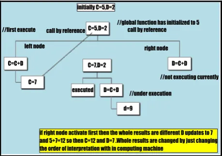
computers are the punched cards then they moves toward vacuumed tubes and then magnetic tapes and then so on .The main thing to note in the evolution is that change occurs to make the system simpler and less complex. The real need of interpretation in field of computing comes after the digitalization of computers, as computers can only understand the language of pulses (binary 0-1) so an interpreter is required to convert the high level language (general) into low level machine language. Interpretation and transmissions are taken as almost one in the same, in early days of the computing machines. As one node is Interpreting and the other node is transmitting and when the other node is transmitting the initial node is interpreting e.g. figure below shows a demo of the procedures with in an inter node interpretation and transmission.

[image:1.595.316.545.379.546.2]

Fig.1: demo of transmission and interpretation [key Board]

(2)

supports "single process single thread" or "multiple processes multiple threads" etc.

Interpretation and transmissions are also dependent on some factors which are listed below

 Transmission Density:

The maximum amount of data that can be sending or received

 Attenuation problem:

The loss in data transmissions and interpretations

 Transmission distortions:

How much the processes are disturbed by the external sources [1].

 Number of End-user:

It is the total no of hops or nodes receiving that data from the transmission channels. Humans also belong to one of the most advance categories of computational machines. As computational machines are constructed keeping in mind the criteria of “EASE OF USE” and they are also developed in the way that they produce a sound image of humans interpretation and transmissions [2]. So we will also through light on human way of interpretation and transmission and its projection on the computing machines in the domain of bio-informatics.

2. SYNCHRONOUS

INTERPRETATIONS AND

TRANSMISSIONS

Two basic requirements must be satisfied when the process interacts with each other that are: synchronization and communication. To produce symmetry with in instruction or data processing is one of the most important tasks, if the culture of data in non-symmetric then it is very hard for us to predict the pattern of data that rather it’s increasing, decreasing or sinusoidal. Finding the signature of a particular pattern is half the success; the other phase of success is to devise a particular and efficient algorithm for that particular system. Once the signature is locked, mathematical function are developed which will help us not only to check the effectiveness of current system but also tell us its efficiency on the “nth” interpretation. Synchronous approach is relatively easy to implement and integrate with the system as you don’t have to worry about the other factors which will affect the mode of transmission [3]. But synchronous communication have some other factor involves in it e.g. until the message is not sent the receiver can’t really receive the message or if they sent the message, until the message sent is being processed they can’t do something else like in old “Nokia” mobiles but modern mobiles do support multi-processing . Synchronous transmissions are easily classified in three states; blocked, initialized and suspended. Keeping in mind the certain characteristics of synchronous transmissions “SEMAPHORES” are developed. Semaphores are just integer notations assigned to the data processing. Only three operations can be performed on particular semaphores which are initialize, increment, and decrement. [4].When we talk about the order of execution, interpretation or transmission them the term “RACE CONDITION” comes into action this is basically a problem while performing the execution of those instructions which uses same global function. E.g. In

[image:2.595.316.546.212.373.2]

programming terms this phenomena is usually referred to as “PASSED BY REFERENCE” if one instruction calls for a function and the passing is by reference then the values in the global variable are up dated, if again a second instruction calls for the same function and do the same computation but now both of the instructions have different results because the first to update its result in the global function and the change becomes permanent. When one instruction goes in the critical section other interrupts and processes are forbidden to call the function. Their requests for function are queued when the processing of the function is done then queue is DE queued and processing is done. This phenomena is called “Mutual Exclusion”

Fig.2: Different results shown by the global function dependent upon the race condition

In order to make our calculations correct we need to keep the track of those changes made by the first instruction calling the function and then allocate or de allocate the resources according to it. Now suppose another scenario: one instruction calls for the global function and suddenly second instruction calls for the same function again and the global function has yet not completed the interpretation of first instruction then what the computational system will do? Who will it serve? So to solve this problem many techniques are introduced one of that technique is to disable any further call for the function when it moves into the critical section. The other one is to define the priorities, if high priority instruction comes, the interpretation of the current instruction temporarily stops the new program counter values are loaded and the service will then be provide to the recently loaded one. After the execution of instruction, old values of PC (program counter) and PSW (process State Word) are loaded back to the memory for the continuation of the existing process.

3. ASYNCHRONOUS

INTERPRETATIONS AND

TRANSMISSIONS

(3)

up” signal is transmitted to the receiving computational device which will then send acknowledgment back to the device sending the data. Start and stop bit are used to insure atomicity of each bit. In simple word asynchronous is a mode of transmission which is non-periodic and non-regular. Each bit has its own starting and stopping point and their output rate is independent of the transmitting computational machine. Asynchronous transmission is non-periodic so it opens gates to some astonishing domain which are listed as under:

3.1 Operating system less Computational

Machines:

As in synchronous transmission devices e.g. take the example of a pc, to properly run any application you must have to boot the system, initially BIOS takes control of the system then the control is transferred to the boot strap loader whose main purpose is to locate the OS starting from the disk, and then boot strap loader passes its control flag to the operating system which will then load itself, then after that you can run any application over it. Suppose you company only wants to work with MS OFFICE so then the question arises that why it should load OS and all its components? Isn’t it causing ambiguity and frustration not only with the clients but also with in the workers? Asynchronization provides answer for that, you don’t need to work with time just put office cd in the system and the integrated drivers do the magic for you. This approach can also be called as “integrated system approach”. Bios comes as integrated to the system so modern scientists in field of computer science are doing research on build an “OS chip” similar to the “BIOS chip”. This provides a major breakthrough in field of computing device. As by now no such system exists. Because the “OS now a days are very much large to fit in a chip”. Only real time systems are being developed using integrated OS approach. If integrated OS technology is applied to normal computing machines then the price of that computational machine is out of the bounds of their customer and hence product goes in loss but real time systems (like anti-missile systems, Radar systems etc.) are developed without bothering about the cost of the system. In real time systems optimum timing and calculation is required, so that they perform the co-ordinates calculation of their target in Nano seconds and make response to the control tower which will arm or dis-arm the system. These systems are very expensive and thus can only be affordable by the governments

3.2 Less Power Consuming Devices:

As the clock pulse and the levels of different type of execution is removed from the system then system becomes efficient and efficiency of that system is not only with respect to the number of steps involves or time of execution of particular instruction but also with respect to power consumed[6]. The system becomes so energy efficient that it can even run on a power as small as that of a potato in its life time.

4. SYNCHRONOUS AND

ASYNCHRONOUS TRANSMISSION

AND INTERPRETATION ANALYSIS:

We have analyzed some synchronous and Asynchronous Activities over AMD Dual Core Process and got some wondering results which are described as under: Initially when any Synchronous transmission is initiated on the processors it will consumes a large amount of processors

speed but the ratio then decreases and decreases to nearly zero then when the threads stops and the new process loads the ratio again rises to its peek value and then start decreasing again. This phenomena is shown in below figure when the synchronous transmission is executed on the core processor

Fig.3: (shows variant behavior of processor while execution of synchronous transmissions)

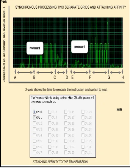
Now we take the same transmission and now the grid plotting is on two different processors using the same AMD processor and then again the results are amazing. Separate grid means each processor plots its separate graph of net utilization. Below figure shows the processors utilization with respect to time on separate boundaries.

Fig.4: (shows variant behavior of processor while execution of synchronous transmissions using separate

[image:3.595.314.541.128.352.2] [image:3.595.319.538.451.734.2]

(4)

At point ‘A’ in the above figure the transmission has been started. Looking at the grid it is evident that any processor can grab the interrupt and start interpreting the transmissions so both A and ‘E’ initially activates them then it’s up to algorithm that either any one or both can start the execution of the transmission In fact processor 0 starts the transmission above but some system processes and threads of current process are transferred to processor 1 to handle them. From point A to B execution of the process starts and up till point B threads load and de-load themselves. From point B to C refreshing of the processors takes place. At point C i have attached affinity to “processor 0” (only one specific processor is allowed to start and stop the transmission other processor is unaware of the transmission) now transmission is bound to processor 0. And it is evident from the above figure that initially both processors almost shows same behavior to the transmission (A-B&E-F) then refreshing is also almost same from (B-C&F-G) the fact that “processor 1” refreshing peak is high because it is less utilized as compared to “processor 0” .At points C-D in processor 0&G-H in processor 1, the difference is evident when we attach affinity to “processor 0” for current transmission then “processor 1” utilization drops to almost zero. Basically when you attach affinity to any process then the process is dependent on the processor to whom it has attached. By default any transmission or interpretation has affinity of both processors.

So an intelligent algorithm can be developed so that it continuously monitors the level and magnitude of transmission and intelligently switch across the affinities so that when a dense process comes in the system the switching is done and the whole processor is dedicated to that process. Thus it will enhance the overall processing time of the system and also increase the worth of the system.

5. PROPOSED SOLUTION TO AN

INTELLIGENT AFFINITY ALLOTTER:

Artificial intelligence is such fascinating fields of computer science that machine mimic the characteristics of human decision making capabilities. It not only removes the human error in making decision but also provides efficient approach to a certain problem.

In automatic affinity allotter initially you ask for the end-user (of multi-processor users) in the installation of operating system that either you want to attach automatic affinity or manual affinity to the processes and threads, obviously normal user prefers automatic affinity but if the automatic affinity is not checked don’t implement automatic affinity and continue with the normal processing.

The steps involved in deciding the process affinity and its allocation to processor are described briefly if the following algorithm:

ALGORITHM: START:

Do you want to attach intelligent affinity allocator to the system?

[Yes/no]

If (answer==’YES’)

Start processing:

Let X is a variable to monitor the density of transmission.

*When the transmission is initialized then X is also initialized transmission=1, x=1

Let ‘\0’ be the end of transmission.

While the threads and the processes of current transmission executes x is incremented until the end of the size of transmission

While (transmission state=execution) X++ up till end of transmission ‘\0’;

If (X++ > =standard Transmission size)

*Standard transmission size can be set by mutual understanding of the system designers and the stake holders of ALLOTER.

Check Processors 0, 1, 2….n

*Where n are maximum processors

Compare the processors and find processor with least processing

*here number of processor = number of variables initialized for calculating the processor which has least processes We suppose 2 processors are initialized processor 0 and processor 1 so two variables are initialized

Initialized A, B If (A< B)

Smallest processing=A; Else if:

Smallest processing =B Else:

Both are equal Return any one. Return smallest processing

*In case of 5 processors the process is as under Initialization…A, B, C, D, E rest of processing is same.

When the processor with lowest utilization is returned interrupt is generated to switch the current transmission to the returned processor or start attaching affinity to the transmission

Returned processor <- transmission Until transmission! = (not equal to) ‘\0’ Else break:

Inner loop exits

Now outer loops (If x++ < standard Transmission size) Continue default execution:

Closing Outer most loop If (answer==’NO’)

Break: END

(5)

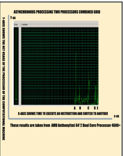
Fig.5: (shows variant behavior of processor while execution of asynchronous transmissions using one

plotting grid)

The same transmission which is previously performed using synchronization now has been done using Asynchronization. Initially at point A both have a high peak as the processes is interpreted by the processor later the usage goes down and down .Then suddenly at point B another processes has been started so initially the processing goes high but later it will fall, similarly to D, E and F, so here the utilization is low and execution is fast because only relevant information is loaded into the block of processor and continuously starting and stopping bit is loaded which increase the net utilization of the processor. The execution or interpretation time using asynchronous is very small but it consumes a lot of space as for each bit you give a starting bit and stopping bit so in the case of memory utilization or systems where memory efficiency is important this technique cause disadvantage instead of giving advantages. So implementation of any technique depend upon the scenarios, either you are developing a system which is time efficient or efficient in terms of memory utilization.

6. CALCULATIONS REGARDING

SYNCHRONOUS VS. ASYNCHRONOUS:

Let α, β represents the synchronization and Asynchronization and processor clock time is denoted by ‘Ω’:

Then ∑ α (synch) =

Wake up+ ∑system processes+ Ω (processors) +Ω (to load) /W (net processes)

Where ‘W’ is the total no of receiving processes to the processors buffer which in our case is always 4 for

synchronous and 2 for asynchronous. Now developing the equation for Asynchronous transmissions:

∑ Β (asyn) =wake up (µ) + stopping bit (Φ)/2(general)

(1+x)^2 *2+x (complete Equation for solving time for transmission)

(In above formula, multiply by 2 for getting total start and stop bits and again + x for getting total time of transmission including start and stop bits) Because in asynchronous transmission there is a starting bit and a stopping bit.

Using the expansions of the sums let’s compare both of them:

The expansion of the sum is described below

Let’s take the absolute values for both synchronous and asynchronous 1µs (microsecond) for all processes:

n=4 for synchronous and 2 for asynchronous (assuming ideal). X is basically Transmission size.

In synchronous transmission there is almost 4 processes leading to the transmission whereas in asynchronous there are just two processes leading to the transmission.so this will tell us how the two are increasing in processing with respect to the process

When (x=2, n=4) applying the expansion series (synchronous)

= [1+8+24…]

∑estimate = 81µs (micro seconds) required for minimal transmission after each increment total processing time increases

When (x, n) = 2 applying the sum expansion series (asynchronous)

(1+x)^2 *2+x = [1+4+4]*2+3

∑estimate= 21(micro seconds) required

=21µs.

℅β (gained) =∑α/∑β

Β (asynchronous) gain = 81/20 =4.05 times faster

This pattern also tells an important thing that initially either using Asynchronization or synchronization the wake up time will be the same. The difference occurs in the aftermath.

7. FURTHER ANALYSIS OF

SYNCHRONOUS VS. ASYNCHRONOUS

INTERPRETATION AND

TRANSMISSIONS

[image:5.595.55.293.69.371.2]

(6)

[image:6.595.317.547.76.283.2]

Table 1. Shows behavior of synchronous and asynchronous for a given transmission size and the time

gained or lost by asynchronous

Size X (1+X)^4(sy nchronous) α

(1+X)^2*2+x (asynchronou s) β

β Gain in performance

0.005 1.020µs 2.025 µs 0.503(times slower than synchronous

0.1 1.46 µs 2.52 µs 0.57(times slower than synchronous)

1 16 µs 9 µs 1.77 times

faster than synchronous

2 81 µs 20 µs 4.05 times

4 625 µs 54 µs 11.5 times

8 6561 µs 170 µs 38.59 times

50 . .

6765201 µs .

.

5252 µs . .

1288.11 times faster than synchronous

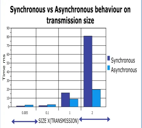
The stats in the below table shows some very important facts. If the size of the transmission is small then synchronous becomes efficient as at X=0.005, using synchronous technique data is transmitted in 1.020 micro seconds whereas Asynchronization takes 2.025 micro seconds, so in this scenario synchronous technique is better than asynchronous. Now let’s take X=8. Using synchronous technique transmission is completed in 6561 micro seconds whereas using Asynchronization transmission is completed in 170 micro seconds. It is evident from those stats that whenever the size of the transmission is small synchronous should be preferred over asynchronous as it makes the overall system slower. When the size of transmission is large then asynchronous provides the optimum technique for the transmission of data.

Fig.6: (Bar chat view of Table 1 plotting transmission size on y-axis and processing time on x-axis which increases by

size of input)

Fig.7: (Performance Gap Between the two techniques)

[image:6.595.61.280.108.432.2] [image:6.595.314.552.297.656.2]

(7)

8. FACTORS EFFECTING

INTERPRETATIONS AND

TRANSMISSION:

Following are the factors which cause effect on the rate of transmissions

8.1 Transmission density:

It is basically the amount of available space for any transmission to be performed or in other terms it is the maximum allotted space for the receiver or sender to upload its transmission. It is a physical restriction to the transmission and it is non- mask able. If the density allocated to a particular transmission channel is 3 Megabyte then optimum density transmission is 3 MB you by any algometric mean can’t exceeds the upper limit defined by the service provider however it can be increased if your frequency is set for the higher band width and this can only be done by the main frame computers or the servers. Same is the case with the uplink or the up speed which is basically the restriction on the interpretation of the transmission. Up speed in normal conditions is basically the density of the signal to take the input from the host node and start its transmission on the servers. [7] In this method restriction are imposed on the signal that it cannot take more data from the node as much as defined by the service provider .e.g. if the service provider has given you the up speed of 2MB per second then the optimum utilization of a second from the sender point of view is 2MB

8.2 Persistence of the transmission

Persistence of transmission is basically the life of the transmission or the time interval up till which the transmission remains in the system securely. Now day’s persistence of the transmission varies from organization to organization. If the signal is of high significance and so is the response from the user then under such circumstances separate servers or work stations are working with the system to provide persistence for the transmission. Persistence some time can also be taken as the availability of the signals to which the transmission media is connected like 24 hour service or 12 hour service. It is fact that during transition in state, the original data is inaccessible, like if the bank is updating the record of the customers then for certain period of time new customers are forbidden to create new account or perform transactions. Now a day back up of websites are available whenever the change are done in database. Later those changes in backup webs are committed or rolled backed etc.

9. CLASSIFICATION OF

TRANSMISSION AND

INTERPRETATIONS:

Transmissions and interpretation are of two kinds multiplexed or dedicated

9.1 Guided Transmission:

During this transmission certain conductors provide medium for communications. Media might be fiber optics or a wire or any other. In this technique optimum transmission is dependent on the path covered by the media.

As V=IR and as the length of the media increases the resistance increases and the conductivity of the media decreases and hence the transmission got effected. Fiber

optics, co-axial and twisted pair are few examples of guided and conducted media.

9.2 Unguided Transmission:

It is basically a type of transmission where you are not dependent on the path. The thing that counts is the strength of the signal at which you are sending your transmission. For example you are making a wireless communication between two cities then if infra-red is the media for the transmission and interpretations, then it is not logically possible because IR have short range and they even can’t pass through a 5mm metallic foil. Blue tooth is an approach also for short distance transmissions. In unguided media interpretations and transmissions, transmissions are performed by means of antennas; antennas might be internal or external. Antennas might be aligned with respect to the transmitters which match the internal frequency with the frequency of the transmitter and then starts its transmission or line of sight is important in those cases. Omni directional approach can also be used where receivers are not pre-defined. Signals are thrown in each direction and many antennas can catch the transmission started by Omni directional transmitter. Mobile infrared, Bluetooth, GPS, Radio, Telephone are some of the examples of the unguided transmissions.

10. CONCLUSIONS:

Computational machine, some systems prefer time efficiency and some prefer space utilization efficiency. They vary from scenario to scenario. The best approach for large size transmission is asynchronous, because they didn’t consumes the whole processing speed for data interpretation and transmission. The data is send inform of small chunks, which enhances the net speed if space is not a point to ponder for the particular system.

(8)

both of them in the system and let the algorithm to decide which one in better in these specified conditions.

11. REFERENCES

[1]. Stefania Gallova, “Contribution to Incomplete and Noisy Information Problem Solving By Artificial Intelligence Principles Applying”, Published in Proceedings of the World Congress on Engineering Volume I, 2010, June 30-July 2, 2010, London, UK. ISBN: 978-988-17012-9-9. ISSN: 2078-0958 PP 21-28.

[2]. Nada M.A.AL Salami, “Genetic System Generation”, Published in World Congress on Engineering and Computer Science (WCECS). Volume I, October 20-22, 2009, San Francisco USA. ISSN: 978-988-17012-6-8, PP: 23-27.

[3]. L. Rodrigues, M.Raynal, “Atomic Broadcast in Asynchronous Crash-Recovery Distribution System”, Proceedings of the 20th International Conference on Distributed Computing Systems (ICDCS 2000), P: 288, April 10-13, 2000.

[4]. Downey, “THE LITTLE BOOK OF SEMAPHORES”.www.greenteapress.com/semaphores.

[5]. Tiago Goncalves, A. Espirito-Santo, B.J.F. Riberio, P.D. Gaspar, “Design of a Learning Environment for Embedded Systems”, Published in Proceedings of the

World Congress on Engineering Volume I, 2010, June 30-July 2, 2010, London, UK. ISBN: 978-988-17012-9-9. ISSN: 2078-0958 PP 172-177.

[6]. Xinirui.Wang, Tien-Fu.Lu, Lei.Chen, “Synchronization and Time Resolution Improvement for 802.11 WLAN OWPT Measurement”, Published in International MultiConference of Engineers and Computer Scientists. Volume I, March 18-20, 2009, Hong Kong. ISBN: 978-988-17012-2-0 PP: 378-383.

[7]. Sundararaman, B., Buy, U., Kshemkalyani, A.D., “Clock Synchronization for Wireless Sensors Net-works : a Survey,” Ad Hoc Networks, V3 , PP:281-323,2005

12. AUTHOR’S PROFILE

Waleed Abrar was born in Rawalpindi, Pakistan, on October 18, 1990. He has completed his B.S degree in Software engineering (BCSE) from Foundation University Islamabad. He has studied from one the best colleges of Pakistan “F.G Sir Syed College, The MALL Rawalpindi Cantt”.