System Progress Estimation in Time based Coordinated
Checkpointing Protocols
P. K. Suri
Dean, Research andDevelopment; Chairman, CSE/IT/MCA, HCTM Technical Campus, Kaithal,Haryana, India
Meenu Satiza
HCTM Technical CampusABSTRACT
A mobile computing system consists of mobile and stationary nodes. Checkpointing is an efficient fault tolerant technique used in distributed systems. Checkpointing in mobile systems faces many new challenges such as low wireless bandwidth, frequent disconnections and lack of stable storage on mobile nodes. Coordinated Checkpointing that minimizes the number of processes to take useless checkpoints is a suitable approach to introduce fault tolerance in such systems. The time-based checkpointing protocol eliminates communication overheads by avoiding extra control messages and useless checkpoints. Such protocols directly accesses stable storage when checkpoints are saved. In this paper a new probabilistic approach for evaluation of the system progress is devised which is suitable for the mobile distribution applications. The system behavior is observed by varying some system parameters such as fault rate, clock drift rate, saved checkpoint time, checkpoint intervals. A validation regarding system progress is made via a simulation technique. The simulation results show that the proposed probabilistic model is well suited for the mobile computing systems.
General Terms
Checkpointing, System progress, Simulation
Keywords
Distributed system, fault tolerance, time-based checkpointing
System progress, consistent checkpoint
1.
INTRODUCTION
Checkpointing is a major technique of fault tolerance system in which state of a process has to be saved in stable storage so that the process can be restarted in case of fault. There are two main categories of checkpointing techniques: (i) coordinated and (ii) uncoordinated checkpointing. In coordinated checkpointing, the processes send the control messages to their dependent processes to save their states at the same time. This results a global consistent state from which the system recovers when a fault occur in the system. In uncoordinated checkpointing, the processes save their states independently. In this type of protocol, during fault occurrence processes rollback to a point of recovery. Recently new type of time based coordinated checkpointing techniques have been introduced which avoid extra coordination messages among dependent processes. The time based approach is based on loosely synchronized timers. The Timer information is piggybacked along application messages. System performance of the time based checkpointing protocols depends on the
application and system’s characteristics such as checkpoint intervals, save checkpoint time, resynchronize time, clock
progress with particular system parametric values. This model shows that how system operations can affect the system performance and the simulation results shows the states at which system perform well with the particular values of defined parameters. A simulation model is also developed to validate the system progress.
1.1
Related work
In 1985, Chandy and Lamport [1] proposed a global snapshot algorithm for distributed systems. The global state is achieved by coordinating all the processors and logging the channel state at the time of checkpointing. Special messages called markers are used for coordination and for identifying the messages originating at different checkpointing intervals. In 1987, Koo-Toueg [5] proposed a two phase Minimum-process Blocking Scheme for distributed system. The consequence of algorithm is a consistent global checkpointing state that involves only the participating processes and prevent live lock problem (A single failure can cause an infinite rollbacks)
In 1996 Ravi Prakash and Mukesh Singhal [11] presented a synchronous non-blocking snapshot collection algorithm for mobile systems that does not force every node to take a local snapshot. They had also proposed a minimal rollback/recovery algorithm in which the computation at a node is rolled back only if it depends on operations that have been undone due to the failure of node(s).
In 1996 N. Neves and W.K.Fuches [9] presented a time based checkpointing protocol which eliminate communication overhead present in traditional checkpointing protocols. The checkpointing protocol was implemented on CM5 and their performance was compared using several applications. In 2001 Guohong Cao and Mukesh Singhal [4] had introduced the concept of “mutable checkpoint” which is neither a tentative checkpoint nor a permanent checkpoint. To design efficient checkpointing algorithms for mobile computing systems the mutable checkpoints can be saved anywhere e.g. the main memory or local disk of MHs. In this way taking a mutable checkpoint avoids the overhead of transferring large amounts of data to the stable storage at MSSs over the wireless network.
In 2002 Chi-Yi Lin et. al. [7] proposed an improved time based checkpointing protocol by integrating the improved timer synchronization technique. The mechanism of time synchronization utilizes the accurate timer in MSSs as an absolute reference. The timers in fixed hosts (MSSs) are more reliable than those in MHs.
system each process takes a soft checkpoint first which is saved in main memory of mobile hosts. If the process is irrelevant to initiator it can be discarded otherwise will be saved in the local disk at a later time as hard checkpoint. As a result the number of disk accesses in mobile hosts can be reduced. The advantage of using time based approach improves the need of explicit coordination message.
In 2006 Men Chaoguang [2] proposed a two-phase time based checkpointing strategy. This eliminates orphan and in-transit messages. In this strategy, the issues of time - based adaptive checkpoint strategy was evaluated which describes about all processes need not to block their computation work and also not to log all messages. In proposed strategy the inconsistency issues are also discussed.
In 2007 Awasthi and Kumar [6] had proposed a probabilistic approach based on keeping track of direct dependencies of processes. Initiator MSS collects the direct dependency vectors of all processes and sends the checkpoint request to all dependent MSSs. This step was taken to reduce the time to collect the coordinated checkpoint. It would also reduce the number of useless checkpoints and the blocking of the processes. The buffering of selective messages at the receiver end and exact dependencies among processes had maintained. Hence the useless checkpoint requests and the number of duplicate checkpoint requests get reduced.
In 2008 Suchistmita Chinara and Santanu Kumar Rath [3] had proposed an energy efficient mobility adaptive distributed clustering algorithm for Mobile ad-hoc Network. In which a better cluster stability and a low maintenance overhead is achieved by volunteer and non volunteer cluster heads. The proposed algorithm is divided into parts like cluster formation, energy consumption model, cluster maintenance. The objective of algorithm is to minimize the re affiliation rate (A changing situation of member node search for another head is called re affiliation) .The simulation Experiment compare the ID of members. A high ID member act as cluster head and cluster maintenance overhead is reduced from time to time.
In 2011 Anil Panghal, Sharda Panghal, Mukesh Rana [10] presented a comprehensive study of the existing techniques namely Checkpoint-based recovery and Log-based recovery. Based on the study they conclude that Log-based recovery techniques which combine checkpointing and logging of nondeterministic events during pre-failure execution are suitable for systems that frequently interact with the outside world. They also conclude that communication-induced checkpointing reduces the message overhead if implemented along with checkpoint staggering can prove to be the best method for recovery in distributed systems
2.
PROBLEM FORMULATION
In this paper a number of time based checkpointing protocols are analyzed. In [9] Neves and Fuchs had given the concept of timers to reduce the communication overhead. They made the following assumptions:
(a) The processes involved in checkpointing have loosely synchronized clocks.
(b) All the processes are approximately synchronized and have a deviation from real time in their local clock timers. The local clock drift rate between the processes being assumed as ρ.
(c) The timer will terminate at most (2ρT/ (1-ρ2) ≈ 2ρT) seconds apart. Here T is the initial timer value. Normally drift rate ρ attains values between 10-5
sec. to 10-8 sec.
(d) The clocks will show a maximum drift of 2NρT after N checkpoint interval.
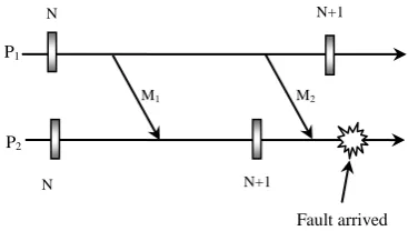
Consider the following figure1. in which P1 and P2 are two
processes. The message M1 is sent from process P1 to P2 in its
Nth checkpoint interval and also message M2 is being sent in
same interval of P1 to (N+1)th interval of P2. Let some fault
arrives in timeline of Process P2.
It is observed that checkpoint N+1 is saved in P2 before the
fault occurrence. Now P2 has yet to receive M2. But P2 has no
information of message M2. Such situations can be handled by
resending unacknowledged messages again.
According to Neves the more time is wasted in storing checkpoints and the processes has to block its execution for a long time which is an impractical situation. Such inconsistencies of in-transit or orphan messages can be handled by using time based checkpointing approach where the messages are now being sent along with timers.
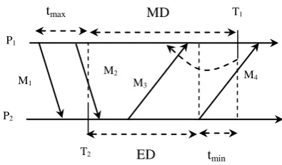
According to Men Chaoguang approach [2] the orphan messages can be eliminated by using communication induced approach and in-transit messages can be stored in message logging queue. The following figure 2. Illustrates the above situations.
Consider P1 and P2 are two processes. T1 and T2 are their
timers respectively. Let MD = D + 2 ρ T be the maximum deviation between the timer of two processes = T1 – T2 .tmax
is the maximum delivery time at which process P2 should get
the message M1. tmin is the minimum delivery time of message
M4. ED = MD – tmin is the effective deviation in which the
processes cannot send or receive the message .M2 and M3 lies
in effective deviation and they arise the inconsistency due to orphan and in-transit messages. To handle orphan message M3
a communication induced checkpoint is placed before the delivery of message M3 and in-transit message M2 can be
retrieved from message logging queue.
It is observed that the parametric values ρ, T, D, tmin, tmax,
fault rate λ, Saved checkpoint point time S, time (t) at which fault occurs affects the mobile distributed system performance.
In this paper a probabilistic model is developed in which the system performance is evaluated by varying various system parametric values.
P1
P2
M1 M2
N N+1
N N+1
[image:2.595.347.531.176.280.2]Fault arrived
3.
SYSTEM PROGRESS EVALUATION
3.1
Probabilistic model development
When faults occur in the system, resynchronization is made. Here the system’s progress is defined as the ratio of constructive computational work to the total work during a given interval of time.
In order to perform a simulation experiment on distributed system a random sample of time t1,t2,t3………..tn is generated by transforming n uniform random numbers u1,u2,u3……un in the interval (0,1). Where λ is the positive constant depending on characteristics of distributed system [12]. The general term of time tk is
tk = – (1/λ)*logeuk where k Є [1,n]
Let ts = time to store checkpoint, tmin be the minimum checkpoint delivery time, tmax be the maximum checkpointing delivery time, Tdiff be the maximum difference between timers of different processes, L be the length of checkpoint intervals before resynchronization, ρ be the clock drift rate between the processes, fr be the fault rate, Tw be the probabilistic wasted time of fault occurrence ,Twr be the probabilistic wasted time of fault occurrence between resynchronization, tr be the resynchronization time.
Let T1, T2, T3………Tnmax are n checkpoint intervals between resynchronization. When fault not occurs then this time will be equal to maximum number of checkpoint intervals nmax.
The system progress is evaluated by developing following probabilistic model.
Here ts ≤ (Tdiff + 2*nmax*L* ρ – tmin)
(ts + tmin – Tdiff)/ (2*L*ρ) ≤ nmax
nmax = ceil ((ts + tmin – Tdiff)/(2*L*ρ)
Let Tcons be the time interval during which constructive computational work is done. Where Tcons is given as
Tcons = L – ts – tk where k Є [1,n]
The probability density function of occurrence of fault is given as
Let Ir = Expected number of intervals between resynchronization = Probability of happening fault during any
Interval less than nmax + Probability of happening no fault during any interval less than nmax.
In Fig. 3 a set of nmax checkpoints numbers ({1, 2, 3 ……k, k+1…nmax}) are considered on the time line of the process.
The probability of a fault occurring in the kth checkpoint interval Pr[k] in last resynchronization process is given as
Pr[k] = e – fr* L*k – e – fr* L*(k+1)
(nmax – 1)
Ir =
∑
k * Pr[k] + nmax * e – fr* L*kk =1
Ir = (1 – e – fr* L*nmax)/ (e fr* L – 1)
Probability of wasted time of occurrence of fault Tw and the wasted time of occurrence between resynchronization Twr is given as
Tw = ((e – fr*Tcons)*( – fr * Tcons – 1 ) + 1)/(fr*(1 – e – fr*Tcons ))
The Probability of wasted time of occurrence between resynchronization Twr is given as
Twr = (1 – e – fr* L*nmax)*( ts +Tw) + e – fr* L*nmax* tr
Let probability of total time between resynchronization is Tr .
Where Tr = Ir * L + Twr
Let TCW be the Probability of time used in constructive work between resynchronization
TCW = Ir*Tcons
The System Progress (SP say) of a process = TCW/Tr
The System Progress of all the processes = ∑ TCW/Tr
The System Progress of the complete system having n processes = (∑ TCW/Tr)/n.
3.2 Validation of system progress
To confirm the correctness of system progress evaluation, system progress validation is implemented to more detailed confidence level of simulation. Here in the simulation technique to achieve the validation having a better confidence level ,first 1000 runs of simulation experiment are made from 10 samples with 100 checkpoint intervals then 2000,3000,……..10000 runs are made and then average value of system progress, their standard deviation (say SD), upper ( say UL) , lower (say LL) confidence limit of system progress is computed. Further corresponding interval of interest Tcons and then corresponding optimal system progress is evaluated for the system by using the variation among the parameters say λ, ρ, ts, fr, L. The used simulation technique follows as Let’s take n independent samples of time interval Length L and according to such n samples values of System progress SP1,SP2,SP3………SPn .Then their mean μ and
P1
P2
M1
tmax
T2
T1
M2
M3
M4
tmin ED
[image:3.595.68.266.83.199.2]MD
[image:3.595.314.543.97.286.2]Fig.2 Elimination of inconsistent state
Fig 3. Fault arrival in kth checkpoint interval L
2
1 k k+1
Fault
Waste
time
standard deviation σ are evaluated .The sample mean of all System progresses are to be evaluated by using formula:
SPmean = ∑ SPi/ n
The variance σ2
can be estimated as :
σ2est = (1/ (n-1))*∑(SPk – SPmean) 2
The general relationship between the parameters is given as
Pr {μ – t ≤ SPmean ≤ μ + t} = 1 – α
where t is the tolerance on either side of mean within which the estimated to fall within probability 1– α. The normal density function is Φ(y) = y1-α/2, the upper confidence limit UL
and lower confidence limit LL of System progress can be obtained respectively.
y
Φ(y) =
∫
(1/√2Π)* e–(z2 /2)*dz
–α
Where z = (√n) *(SPmean – μ)/ σest
UL = SPmean + (y1-α/2* σest) / (√n)
LL = SPmean – (y1-α/2* σest) / (√n)
y1-α/2 = 2.58 (99% confidence level)
The interval (UL - LL) will contain the true mean with a specific certain experimental confidence value [12].
3.2
Simulation results
Simulation result shows that the System Performance is affected by the various factors such as number of checkpoint intervals, Clock drift rate of processors, Fault rate of processors, Time of saving checkpoints .In our simulation experiment such variations of factors against System Progress are shown in tabular as well as graphical form.
3.2.1
Checkpoint interval vs. system progress
The following table expresses the parametric values used in proposed model. The first column shows when varying values of Fault rate (Table 4), Drift rate (Table 5), Checkpoint intervals (Table 2) and second and third column shows the corresponding other variable names and their particular values.
Table 1: Parametric values of System model
[image:4.595.344.514.161.390.2]
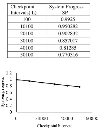
According to these values the system progress is evaluated and respective graphs are drawn. First according to increasing values of checkpoint intervals (L) corresponding decreasing values of system progress is evaluated i.e. obviously as number of checkpoint intervals are increased corresponding system progress get decreased (Fig 4) i.e. The system progress is affected by number of checkpoints
Table 2. Checkpoint intervals vs. System Progress
Checkpoint Intervals( L)
System Progress SP
100 0.9925
10100 0.950282
20100 0.902832
30100 0.857017
40100 0.81285
[image:4.595.56.229.252.340.2]50100 0.770316
Fig 4: Checkpoint intervals vs. System Progress
3.2.2
Saved Checkpoint time vs. system progress
Table 3. describes as time to save checkpoints get increased the system progress get decreased.
[image:4.595.347.509.509.731.2]This is illustrated in Fig.5 which is obviously true as the time to save checkpoint get increased the system progress will decrease.
Table 3. Saved Checkpoint time vs. System Progress
Saved checkpoint Time (ts)
System Progress (SP)
1 0.98183
2 0.981554
3 0.981278
4 0.980999
5 0.980723
6 0.980441
7 0.980166
8 0.979887
9 0.979609
10 0.979331
11 0.979053
12 0.978775
13 0.978498
14 0.978221
15 0.977942
SYSTEM PROGRESS EVALUATION Used System parameters
Variable tr 0.1
State Tdiff 0.01
tmin 0.001
fr L 3600
Fault rate ts 0.7
ρ 0.000001
ρ fr 0.00001
Drift rate L 3600
ts 0.7
L fr 0.00001
Ckeckpoint
Interval ρ 0.000001
Fig 5: Checkpoint intervals vs. System Progress
3.2.3
Fault Rate vs. system progress
This subsection describes how fault rate affects the system progress.
[image:5.595.345.517.98.379.2]Table 4. describes as fault rate get increased The system progress get decreased.This is illustrated in Fig.6
Table 4. Fault Rate vs. system progress
Fault Rate fr
System Progress SP 1.00E-16 0.999803
1.00E-15 0.999741
1.00E-14 0.999767
1.00E-13 0.999783
1.00E-12 0.999802
1.00E-11 0.999761
1.00E-10 0.999726
1.00E-09 0.999765
1.00E-08 0.999658 1.00E-07 0.999625
Fig 6 Fault Rate vs. System Progress
3.2.4
Drift Rate vs. system progress
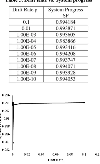
This subsection describes how drift rate affects the system progress. For low value of drift rate the system progress is high little bit .The System Progress of non blocking protocol is not much affected for different values of drift rate the System .Table 5. and Fig.6 illustrates this.
Table 5. Drift Rate vs. System progress
Drift Rate ρ System Progress SP
0.1 0.994184
0.01 0.993871
1.00E-03 0.993605 1.00E-04 0.983866 1.00E-05 0.993416 1.00E-06 0.994208 1.00E-07 0.993747 1.00E-08 0.994071 1.00E-09 0.993928 1.00E-10 0.994053
Fig 7 Drift Rate vs. System Progress
3.2.5
System progress validation
In Table 6. the first column, first entry illustrates that 10 samples of checkpoint interval of length 100 are taken and corresponding System progress of 100,200,…..1000 checkpoint intervals gets evaluated, their average is shown in second column (i.e. 0.99520).The third and fourth column shows their standard deviation, upper and lower confidence limit respectively. Similarly System Progress of other samples having checkpoint intervals 2000, 3000 …10000 are validated
Similar validation can be applied to other system parameters. The difference between upper and lower confidence limit should be less than 2*Tolerance value. Here tolerance value is
[image:5.595.81.248.296.618.2]0.001 for 99% confidence
Table 6. System progress validation
Sample No.
System Progress average
σest
Upper Confidence. Limit
Lower Confidence Limit 1000 0.99520 0.00114 0.9961 0.99427
2000 0.99180 0.00141 0.9929 0.99065
3000 0.98702 0.00146 0.9882 0.98583 4000 0.98215 0.00014 0.9833 0.98095
5000 0.97727 0.00014 0.9784 0.97606
6000 0.97238 0.00147 0.9735 0.97117 7000 0.96750 0.00147 0.9687 0.96629
8000 0.96263 0.00147 0.9638 0.96143
9000 0.95777 0.00146 0.9589 0.95658
[image:5.595.93.241.306.488.2] [image:5.595.315.543.566.743.2]4.
CONCLUSION
In this paper the problem of arrival of fault is efficiently discussed. A probabilistic model is developed for evaluation of System progress of the processes along with a particular set of parameters. It is observed that the System Progress is evaluated by introducing the time generated by negative exponential distribution function. The system Progress gets optimizes on particular values of system parameters. A validation regarding the System progress on the basis of set of parameter checkpoint interval length (L) value is derived .Such validation can be evaluated regarding the other set of parameters such as drift rate, fault rate, saved checkpoint
time
.
5.
ACKNOWLEDGMENTS
Sincere thanks to HCTM Technical Campus Management Kaithal-136027, Haryana, India for their constant encouragement.
6.
REFERENCES
[1] Chandy K.M. and Lamport L. “Distributed Snapshots: Determining Global States of Distributed Systems” ACM Transactions Computer systems vol. 3, no.1. pp. 63-75, Feb.1985
[2] Chaoguang M., Yunlong Z. and Wenbin Y., “A two-phase time-based consistent checkpointing strategy,” in Proc. ITNG’06 3rd IEEE International Conference on Information Technology: New Generations, April 10-12, 2006, pp. 518–523.
[3] Chinara Suchistmita and Rath S.K.“An Energy Efficient Mobility Adaptive Distributed Clustering Algorithm for Mobile ad-hoc Network” 978-1-4244-2963-9/08 (2008) IEEE.
[4] Guohong Cao and Singhal Mukesh, “Mutable Checkpoints: a new checkpointing approach for Mobile Computing Systems”, IEEE Transaction on Parallel and
Distributed Systems, vol. 12, no. 2, pp. 157-172, February 2001
[5] Koo. R. and Toueg. S. “Checkpointing and Rollback-Recovery for Distributed Systems”. IEEE Transactions on Software Engineering, SE-13(1): pp 23-31, January 1987.
[6] Kumar Lalit, Kumar Awasthi, “A Synchronous Checkpointing Protocol for Mobile Distributed Systems: Probabilistic Approach” International Journal of Information and Computer Security, Vol.1, No.3 .pp 298-314, 2007.
[7] Lin C., Wang S., and Kuo S., “A Low Overhead Checkpointing Protocol for Mobile Computing System” in Proc of the 2002 IEEE Pacific Rim International Symposium on dependable computing (PRDC’02).
[8] Lin C., Wang S., and Kuo S., “An efficient time-based checkpointing protocol for mobile computing systems over wide area networks,” in Lecture Notes in Computer Science 2400, Euro-Par 2002, Springer-Verlag, 2002, pp. 978–982. Also in Mobile Networks and Applications, 2003, vo. 8, no. 6, pp. 687–697.
[9] Neves N., Fuchs W.K., “Using time to improve the performance of coordinated checkpointing,” In: Proceedings of 2nd IEEE International Computer Performance and Dependability Symposium, Urbana-Champaign, USA, 1996, pp.282 –291.
[10]Panghal Anil, Panghal Sharda, Rana Mukesh “Checkpointing Based Rollback Recovery in Distributed Systems” Journal of Current Computer Science and Technology Vol. 1 Issue 6 [2011]258-266.
[11]Prakash R. and Singhal M., “Low-Cost Checkpointing and Failure Recovery in Mobile Computing Systems”, IEEE Transaction on Parallel and Distributed Systems, vol. 7, no. 10, pp. 1035-1048, October1996.