Modified Logistic Maps for Cryptographic Application

http://dx.doi.org/10.4236/am.2015.65073

Modified Logistic Maps for Cryptographic

Application

Shahram Etemadi Borujeni, Mohammad Saeed Ehsani

Faculty of Computer Engineering, University of Isfahan, Isfahan, Iran Email: [email protected], [email protected]

Received 13 October 2014; accepted 7 May 2015; published 12 May 2015

Copyright © 2015 by authors and Scientific Research Publishing Inc.

This work is licensed under the Creative Commons Attribution International License (CC BY).

http://creativecommons.org/licenses/by/4.0/

Abstract

In this paper, definition and properties of logistic map along with orbit and bifurcation diagrams, Lyapunov exponent, and its histogram are considered. In order to expand chaotic region of Logis-tic map and make it suitable for cryptography, two modified versions of LogisLogis-tic map are proposed. In the First Modification of Logistic map (FML), vertical symmetry and transformation to the right are used. In the Second Modification of Logistic (SML) map, vertical and horizontal symmetry and transformation to the right are used. Sensitivity of FML to initial condition is less and sensitivity of SML map to initial condition is more than the others. The total chaotic range of SML is more than others. Histograms of Logistic map and SML map are identical. Chaotic range of SML map is fivefold of chaotic range of Logistic map. This property gave more key space for cryptographic purposes.

Keywords

Chaotic Map, Modified Logistic Map, FML Map, SML Map

1. Introduction

In order to explain simple chaotic dynamical systems, one-dimensional map is used. Tent, Bernoulli and Logis-tic maps are common examples of them. The return map of Tent and Bernoulli are linear, while LogisLogis-tic map is nonlinear [1]-[3].

plain by a recursive function as follows:

(

)

(

)

1 , 1

n n n n

x+ =L r x = ⋅ ⋅ −r x x (1)

where r is its parameter and xn∈

[ ]

0,1 . Consider Logistic map L: 0,1

[ ] [ ]

→ 0,1 , given by Equation (1), the pa-rameter r lies in interval

[ ]

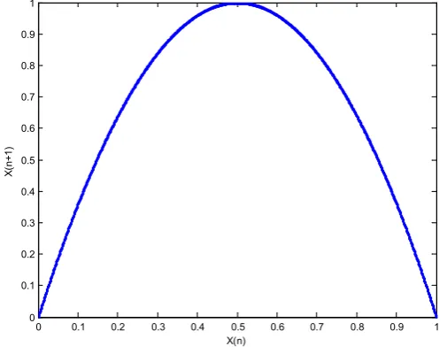
0,4 . The return map of Logistic function is given inFigure 1 for r=4.

Sensitivity of Logistic map to initial condition could be observed by plotting orbit diagrams with respect to two initial conditions with small difference. The corresponding orbit diagrams with respect to two initial condi-tions 0.350 and 0.351 for fixed values of r=4 is drawn in Figure 2. There is suitable sensitivity to initial condition.

In order to view chaotic properties of Logistic map, bifurcation diagram and Lyapunov exponent of it should be calculated and plotted. Bifurcation diagram of Logistic mapwith respect to “r”are calculated and plotted in

Figure 3.

Lyapunov exponent of Logistic mapwith respect to “r”are also calculated and plotted inFigure 4. Regarding

Figure 3 andFigure 4, Logistic map is chaotic when parameter “r” lies in interval [3.6, 4]. First, confirm that you have the correct template for your paper size.

3. Modified Logistic Maps

[image:2.595.187.440.505.705.2]

A discrete dynamic process is said to be two-segmental if there exists a partitioning point. The general equation

Figure 1. Return map of logistic map with respect to r = 4.

0 0.1 0.2 0.3 0.4 0.5 0.6 0.7 0.8 0.9 1 0

0.1 0.2 0.3 0.4 0.5 0.6 0.7 0.8 0.9 1

X(

n+

1)

[image:3.595.194.429.83.273.2] [image:3.595.200.428.313.492.2]

Figure 2. Orbit diagrams of logistic map with respect to two initial conditions 0.350 and 0.351 (r = 4).

Figure 3. Bifurcation diagram of logistic map with respect to r.

Figure 4. Lyapunov Exponent of Logistic map with respect to r.

0 2 4 6 8 10 12 14 16 18 20

0 0.1 0.2 0.3 0.4 0.5 0.6 0.7 0.8 0.9 1

n

X

(n

)

x=0.350 x=0.351

0 0.5 1 1.5 2 2.5 3 3.5 4

0 0.1 0.2 0.3 0.4 0.5 0.6 0.7 0.8 0.9 1

0 0.5 1 1.5 2 2.5 3 3.5 4

[image:3.595.196.429.520.706.2]

( )

n n

(

1 n

)

, n .

h x = ⋅ ⋅ −r x x x ≥a



Considering Equation (4), the derivatives of g x

( )

is exceeding unity, but this is not true for h x

( )

. To solve this problem, we use symmetry and transform properties to modify h x

( )

. Actually, we modified second part of Logistic map in order to improve chaotic range of Logistic map in two manners.

3.1. First Modified Logistic (FML) Map

We modified Logistic map, by obtaining vertical symmetry of g x

( )

around y r= 8, then transform the result to right for x=0.5, to generate a new h x

( )

.The recursive equation of First Modified Logistic (FML) map is defined in Equation (5), where n is a time index, x0 is the initial value, and r is the control parameter.

(

)

_{( )}

( )

₍

(

_{) (}

)

₎

1

1 , 0.5;

FML ,

0.5 1.5 4. 0.5.

n n n n

n n

n n n n

g x r x x x

x r x

h x r x x r x

+

 = ⋅ ⋅ − <



= =  _{= ⋅ − ⋅ − + ≥}

 (5)

where xn∈

[ ]

0,1 , r∈

(

0,4

]

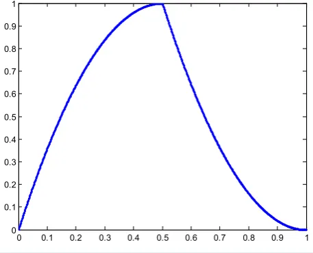
. The return map of the result is drawn inFigure 5 for r=4.

Orbit diagrams of FML map with respect to two initial conditions 0.350 and 0.351 for fixed values of r=4 are drawn inFigure 6. Sensitivity of FML map to initial condition is observed in the graph. There is not suitable sensitivity to initial condition.

[image:4.595.198.427.521.706.2]

Bifurcation diagram of FML map with respect to “r”are calculated and plotted inFigure 7. Lyapunov expo-nent of FML map with respect to “r”are calculated and plotted inFigure 9. According toFigure 7 andFigure 8, FML map is chaotic when parameter “r” lies in intervals [2.6, 2.9] or [3.2, 4].

Figure 5. Return map of FML map with respect to r = 4. 0 0.1 0.2 0.3 0.4 0.5 0.6 0.7 0.8 0.9 1 0

[image:5.595.199.427.82.266.2] [image:5.595.199.428.306.492.2]

Figure 6. Orbit diagrams of FML map with respect to initial conditions 0.350 and 0.351 (r = 4).

Figure 7. Bifurcation diagram of FML map with respect to r.

Figure 8. Lyapunov exponent of FML map with respect to r.

0 2 4 6 8 10 12 14 16 18 20

0 0.1 0.2 0.3 0.4 0.5 0.6 0.7 0.8 0.9 1

n

X

(n

)

x=0.350 x=0.351

0 0.5 1 1.5 2 2.5 3 3.5 4

0 0.1 0.2 0.3 0.4 0.5 0.6 0.7 0.8 0.9 1

0 0.5 1 1.5 2 2.5 3 3.5 4

[image:5.595.199.426.521.704.2]

nent of SML map with respect to parameter ‘r’are calculated and plotted inFigure 12. According toFigure 11

[image:6.595.197.429.297.695.2]

andFigure 12, SML map is chaotic when parameter ‘r’ lies in intervals [2, 4].

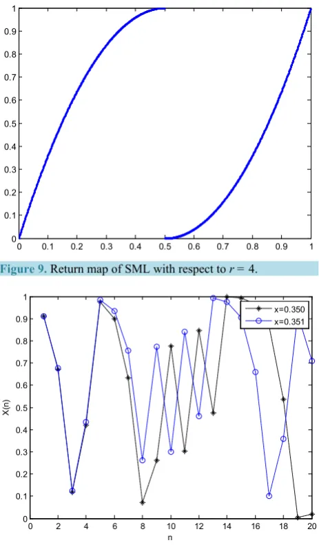
Figure 9. Return map of SML with respect to r = 4.

Figure 10. Orbit Diagrams of SML map with respect to initial conditions 0.350 and 0.351 (r = 4).

0 0.1 0.2 0.3 0.4 0.5 0.6 0.7 0.8 0.9 1 0

0.1 0.2 0.3 0.4 0.5 0.6 0.7 0.8 0.9 1

0 2 4 6 8 10 12 14 16 18 20

0 0.1 0.2 0.3 0.4 0.5 0.6 0.7 0.8 0.9 1

n

X

(n

)

[image:7.595.197.427.84.490.2]

Figure 11. Bifurcation diagram of SML map with respect to r.

Figure 12. Lyapunov exponent of SML map with respect to r.

4. Comparison

With the purpose of expanding chaotic range, two modified version of Logistic map are proposed. In order to compare the performance of the proposed maps with respect to applications, orbit diagrams, bifurcation diagram, Lyapunov exponent and histogram of outputs are considered. Orbit diagram shows the sensitivity of the map to initial conditions. Bifurcation diagram and Lyapunov exponent is used to evaluate chaotic behavior of the maps. Histogram of outputs which could be plotted by observing outputs of large number of iterations, simulate proba-bility density function of the maps.

4.1. Sensitivity to Initial Condition (Orbit Diagram)

In order to compare the sensitivity of the proposed maps, FML and SML, with Logistic map to initial condition, their orbit diagrams with respect to two initial conditions with small difference are considered. They are shown inFigure 2,Figure 6 andFigure 10, respectively. As it explained earlier, sensitivity of FML to initial condition is less and sensitivity of SML map to initial condition is more than the others.

4.2. Chaotic Range (Bifurcation Diagram, Lyapunov Exponent)

Bifurcation diagram and Lyapunov exponent of Logistic mapwith respect to “r”are plotted in plottedFigure 3

andFigure 4, respectively. Meanwhile, bifurcation diagram and Lyapunov exponent of FML map are also plot-

0 0.5 1 1.5 2 2.5 3 3.5 4

0 0.1 0.2 0.3 0.4 0.5 0.6 0.7 0.8 0.9 1

0 0.5 1 1.5 2 2.5 3 3.5 4

5. Conclusions

In order to evaluate the performance of Logistic map, after considering definition and properties of it, orbit dia-grams, Lyapunov exponent and histogram of Logistic map were considered. Orbit diagram showed that the sen-sitivity of Logistic map to initial condition was medium. Bifurcation diagram and Lyapunov exponent were used to evaluate chaotic properties of the map and recognize the range of parameters. The total chaotic range of Lo-gistic map was small.

[image:8.595.197.430.418.702.2]

With the purpose of expanding chaotic range, two modified versions of Logistic map are proposed. They are one-dimensional and two-segmental nonlinear maps. We called them First and Second Modified Logistic (FML & SML). We found vertical symmetry of first segment, transformed the result to right for the second segment, and called it FML map. Definition and properties of FMLmap were also considered. Sensitivity of FML map to

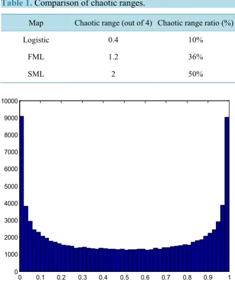
Table 1. Comparison of chaotic ranges.

Map Chaotic range (out of 4) Chaotic range ratio (%)

Logistic 0.4 10%

FML 1.2 36%

SML 2 50%

Figure 13. Histogram of logistic map iterations for r = 4. 0 0.1 0.2 0.3 0.4 0.5 0.6 0.7 0.8 0.9 1 0

[image:9.595.199.426.86.282.2]

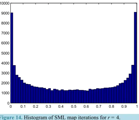
Figure 14. Histogram of SML map iterations for r = 4.

initial condition is not suitable. However, FML map is chaotic when parameter “r” lies in intervals [2.6, 2.9] or [3.2, 4] according to the graphs of bifurcation diagram and Lyapunov exponent. To define a second version-modified Logistic map, we found vertical and horizontal symmetry of its first segment and transformed the re-sult to right. Recursive equation of Second Modified Logistic (SML) map is forming. Sensitivity of SML map to initial condition is observed in the figure. There is superior sensitivity to initial condition. According toFigure 11 andFigure 12, SML map is chaotic when parameter “r” lies in intervals [2, 4].

It was concluded that sensitivity of FML to initial condition was less and sensitivity of SML map to initial condition was more than the others. Histograms of Logistic map and SML map are identical, while FML map cannot perform acceptable results. The total chaotic range of SML is more than the others. Chaotic range of SML map is fivefold of chaotic range of Logistic map. This property expands key space for cryptographic pur-poses.

References

[1] Alligood, K., Sauer, T. and Yorke, J. (1996) Chaos: An Introduction to Dynamical Systems. Springer-Verlag, New York.

[2] Strogatz, S. (1994) Nonlinear Dynamics and Chaos. Perseus Books, Cambridge.

[3] Schuster, H.G. and Just, W. (2005) Deterministic Chaos: An Introduction. 4th Edition, WILEY-VCH Verlag GmbH, Weinheim. http://dx.doi.org/10.1002/3527604804

[4] Li, S., Li, Q., Li, W., Mou, X. and Cai, Y. (2001) Statistical Properties of Digital Piecewise Linear Chaotic Maps and Their Roles in Cryptography and Pseudo-Random Coding. Cryptography and Coding, 2260, 205-221.

http://dx.doi.org/10.1007/3-540-45325-3_19

[5] Addabbo, T., Alioto, M., Bernardi, S., Fort, A., Rocchi, S. and Vignoli, V. (2004) The Digital Tent Map: Performance Analysis and Optimized Design as a Source of Pseudo-Random Bits. Proceedings of the 21st IEEE Instrumentation and Measurement Technology Conference, IMTC 04, 2, 1301-1304.

[6] Addabbo, T., Alioto, M., Bernardi, S., Fort, A., Rocchi, S. and Vignoli, V. (2004) Hardware-Efficient PRBGs Based on 1-D Piecewise Linear Chaotic Maps. Proceedings of the 11th IEEE International Conference on Electronics, Cir-cuits and Systems, ICECS 2004, 13-15 December 2004, 242-245.

[7] Pareek, N., Patidar, V. and Sud, K. (2010) A Random Bit Generator Using Chaotic Maps. International Journal of Network Security, 10, 32-38.

[8] Shastry, M., Nagaraj, N. and Vaidya, P. (2006) The B-Exponential Map: A Generalization of the Logistic Map, and Its Applications in Generating Pseudo-Random Numbers. eprint arXiv.org:cs/0607069.

[9] Basios, V., Forti, G.L. and Gilbert, T. (2009) Statistical Properties of Time-Reversible Triangular Maps of the Square.

Journal of Physics A: Mathematical and Theoretical, 42, 1-13. http://dx.doi.org/10.1088/1751-8113/42/3/035102 [10] Huang, W. (2005) Characterizing Chaotic Processes That Generate Uniform Invariant Density. Chaos, Solitons &

Frac-tals, 25, 449-460. http://dx.doi.org/10.1016/j.chaos.2004.11.016

0 0.1 0.2 0.3 0.4 0.5 0.6 0.7 0.8 0.9 1 0