An Evaluation of Methods for Combining Univariate Time Series Forecasts

(1)

Combining Univariate Time Series

Forecasts

Magnus Svensson

Bachelor’s thesis in Statistics 15 ECTS credits April 2018 Supervised by Jonas Wallin Department of Statistics Lund University

(2)

Abstract

This thesis presents and evaluates nineteen methods for combining up to eleven au-tomated univariate forecasts. The evaluation is made by applying the methods on a dataset containing more than 1000 monthly time series. The accuracy of one period ahead forecasts is analyzed. Almost 3.2 million forecasts are evaluated in the study. Methods that are using past forecasts to optimally produce a combined forecast are included, along with methods that do not require this information. A pre-screening procedure to get rid of the poorest performing forecasting methods before the remaining ones are combined is evaluated.

The results confirm that it is possible to achieve a superior forecast accuracy by combining forecasts. The best methods that utilize past forecasts tend to outperform the best methods that are not considering this data. Including a pre-screening procedure to remove inferior forecasts before combining forecasts from the top five ranked methods seems to increase the forecast accuracy. The pre-screening procedure consists of ranking the automated univariate forecasting methods using an independent, but relevant, dataset. The four best performing methods utilize the pre-screening procedure together with past forecasts to optimally combine forecasts. The best method computes the historical mean squared error of each individual method and weights them accordingly. Demand for automated procedures is growing as the size of datasets increases within organizations. Forecasting from a large set of time series is an activity that can take advantage of automated procedures. However, choosing which forecasting method to use is often problematic. One way of solving this is by combining multiple forecasts into a single forecast.

Keywords: time series forecasting, combining forecasts, M3-Competition, forecast accuracy, evaluation study

(3)

1 Introduction

1.1 Background

Gathering and usage of data has increased rapidly within many sectors of society during the last couple of decades. A prerequisite when working with large datasets is that more or less automatic processes are available. This is especially true when data is updated, or added, frequently. A typical case is forecasting from a large set of time series. Manual forecasting, where an analyst goes through each time series, one at a time, and computes the forecast, is a demanding and time consuming activity. When working with large datasets it is sometimes even impossible to perform this kind of manual work without adding extra labor. The main reason for this is that the time interval between two forecasts being computed is so short that the analyst, or group of analysts, cannot handle all time series before it’s time to start the next round of forecasting, since new information is now available.

Univariate time series forecasting methods are often the first step when forecasts are to be computed. These methods usually require no or little understanding of exogenous data that may be associated with the time series in question. However, they can serve as an alternative to more advanced time series models where in-depth domain knowledge is required to understand practical and theoretical relationships between the analyzed time series and correlated data. Univariate time series forecasting models might be especially attractive when the forecast horizon is short.

Automated univariate time series forecasting methods is not a new thing and has been around in different forms for some time. Their availability and ease of use have increased lately. Several automatic, or semi-automatic, time series forecasting functions are available through the programming language R (R Core Team 2017). Choosing a single automated forecasting method as a starting point is complicated because no method is best in all situations. Bates and Granger (1969) argued almost 50 years ago that combining forecasts from different methods would outperform the individual forecast methods themselves. Suppose, for example, that f1 and f2 are forecasts from

two different methods which are independent and have the same variance σ2. The mean forecast of them is simply fmean = 1₂(f1+f2) and the corresponding variance for fmean is 1₂σ2 which is less than the variance of each individual forecast method. The results from a meta-analysis conducted by Clemen (1989) indicates that this strategy is advantageous.

(5)

1.2 Aims

The primary aim of this thesis consists of evaluating methods for combining forecasts from different univariate time series forecasting methods with the wish of achieving a better forecasting accuracy than the individual methods themselves. The evaluation include forecasts for one period ahead only. The M3-Competition dataset described in Makridakis and Hibon (2000) is utilized in order to evaluate the different methods.

Additional questions related to the main topic are in scope as well. Are methods that are using past forecasts to find an optimal combined forecast performing better than methods that are not? And for these methods, is the forecast accuracy increasing as more past forecasts are included in the process? Is it wise to include a pre-screening procedure to get rid of the poorest performing forecasting methods, before the remaining are combined? These are questions that this thesis aims to provide guidance on.

2 Methods

This section consists of four subsections. The first section describes the automated univariate time series forecasting methods, or procedures, that generate the forecasts that are then combined. The second section describes methods for combining forecasts when past forecasts are not required. This is referred to as methods without training in this thesis. The third section describes methods when past forecasts are utilized, i.e. with training. The fourth section presents methods for evaluating forecast accuracy. A joint annotation of a particular time series is introduced here. Actual values from a time series is denoted as yt for the time periods t = 1, . . . , n. The correspondning point forecast is denoted ˆyt or ft(j) interchangeably, where the latter emphasize from

which of the j = 1, . . . , k univariate forecast methods it is referring to when needed. It should be noted that an even more distinct annotation of ˆyt is by relating it to the time period from which the forecast was made. This means that ˆyt+h is a simplification of writing ˆyt+h|t where information about the forecast horizon h= 1, . . . , mis provided. The notation ˆyt+h|t should be read as the forecast for period t+h produced by using information up until and including period t. Since the focus in this thesis is only on the one step ahead forecasts, i.e. when h= 1, this annotation is relaxed in the text going forward but it should be noted that ˆyt is in fact referring to ˆyt|t−1.

(6)

2.1 Automated univariate time series forecasting methods

The univariate forecasting methods are briefly described in this section. All methods are available as functions via the R programming language (R Core Team 2017). All functions we refer to are set to use default settings except in cases where it explicitly is stated differently. The main interest is to evaluate the difference in forecast accuracy between the univariate and the combined forecasting methods, and this relation is likely not affected by using the default settings. The versions of the referred to R packages are provided in the references.

2.1.1 Fit best ARIMA model

The auto.arima function found in the forecast package (Hyndman 2017) is an auto-mated procedure to estimate a best autoregressive integrated moving average (ARIMA) model according to an information criteria and a testing scheme. The methodology behind the procedure is described in Hyndman and Khandakar (2008). A common obstacle when using ARIMA models for forecasting is to select the appropriate parame-ters because it is usually considered subjective (Hyndman and Khandakar 2008). The auto.arima function tackles this problem by automatically selecting the best number of time lags of the autoregressive model, the degree of differencing needed to reach stationarity as well as the order of the moving average model. This is done on the non-seasonal part and, if appropriate, a seasonal part as well. This method is hereafter referred to as auto.arima.

2.1.2 Exponential smoothing state space model

Various kinds of exponential smoothing techniques for forecasting have been around since at least the 1950s (Hyndman et al. 2002). However, a common framework for model selection within the exponential smoothing family appeared much later. One of these framework is described by Hyndman et al. (2002) and named by the authors as the state space model for exponential smoothing. This family contains methods with different error type, trend type and seasonality type (ETS). Familiar methods as, for example, simple exponential smoothing, Holt’s linear method as well as additive and multiplicative Holt-Winters’, respectively, are included in the common framework together with less well known methods. These most common methods, within the ETS framework, are described in textbooks on time series analysis such as Bowerman, O’Connell, and Koehler (2005). A detailed view of the complete state space framework is given in Hyndman (2008). Theetsfunction found in the forecast package (Hyndman

(7)

2017) is an automatic forecasting procedure that tries models within the state space framework and selects a best method based on an information criteria. This method is hereafter referred to as ets.

2.1.3 Theta method

The theta forecasting method was first mentioned by Assimakopoulos and Nikolopoulos (2000) and is described by the authors as a concept of modifying the local curvature of the time series through the coefficient they call “Theta”, which is directly applied to the second difference. Hyndman and Billah (2003) derived that forecast obtained via the theta method is equivalent to simple exponential smoothing with drift. An implementation of the method is available via thethetaffunction found in the forecast package (Hyndman 2017).

2.1.4 Neural network time series forecast

A neural network model can be fitted to a time series with lagged values of the time series as input. Forecasts can then be made from this model. The neural network model, in this way, is basically a nonlinear autoregressive model. A feed-forward neural network, with a single hidden layer, can be fitted via thennetar function found in the forecast package (Hyndman 2017). A brief introduction to feed-forward neural networks can be found in for example Ripley (1996). This method is hereafter referred to as nnetar.

2.1.5 Simple exponential smoothing forecast

A simple exponential smoothing model (SES) is a very simple way to produce forecasts. Many introductory textbook, like Bowerman, O’Connell, and Koehler (2005), describes this method. A SES model can easily be estimated through the sesfunction found in the forecast package (Hyndman 2017). The sesfunction also includes an automatic optimization rule for selecting the value needed in the initialization phase along with the smoothing parameter. A SES model is in general suitable for forecasting time series without a trend or a seasonal pattern but for a short forecast horizon this might not be a big problem, and this is the reason why this method is included. Also worth noting is that the ets function might select a similar, or even identical, model to what is computed via theses function. The SES method computed through theses function is simply referred to as ses from here on.

(8)

2.1.6 “Prophet” forecast

A recent automated forecasting procedure was presented by Taylor and Letham (2017b), employees at Facebook at the time of release. The procedure is, at its centre, an additive regression model with non-linear trends, including automatic change-point detection, and yearly and weekly seasonality, plus holiday’s adjustments. The procedure is mainly for time series on a daily frequency level and at least one year of historical data but it can be utilized with time series on other frequencies as well (see “Non-Daily Data | Prophet” 2018). The forecast procedure is available through theprophet function found in the prophet package (Taylor and Letham 2017a).

2.1.7 Multiple Aggregation Prediction Algorithm

Multiple Aggregation Prediction Algorithm (MAPA) is a time series forecasting method introduced and described in detailed by Kourentzes, Petropoulos, and Trapero (2014). The algorithm starts with constructing multiple time series, through temporal aggrega-tion, based on the original time series. If for example the original time series consists of monthly observations then bimonthly, quarterly and yearly observations can be com-puted through, temporal, aggregation. Each one of the newly constructed time series could now be forecasted separately. This is done via a similar exponential smoothing framework described earlier as ETS. The last step is then to construct one final forecast by combining the forecasts made from the time series with different frequencies. The MAPA forecasting method is available through the MAPA package (Kourentzes and Petropoulos 2017) and its functions mapaestand mapafor.

2.1.8 Forecasting with temporal hierarchies

Temporal Hierarchical Forecasting (thief) is similar to MAPA since the idea is to take a seasonal time series and compute all possible non-overlapping temporal aggregations, i.e. a monthly time series is aggregated to bimonthly, quarterly, 4-monthly, biyearly and yearly and each of these are then forecasted (see Athanasopoulos et al. 2017). The forecasts are then combined using the hierarchical reconciliation methodology described in Athanasopoulos et al. (2017). According to the authors, the proposed methodology is independent of the forecasting models fitted on the temporal aggregated time series, i.e. they could be based on ETS framework, automatic ARIMA, Theta model or something else; it is up to the user. The thief forecasting algorithm is available in the thief package (Hyndman and Kourentzes 2018) and the function thief. The

(9)

thief method utilized here is using ETS forecasts on the temporal aggregated time series and the method is therefore referred to as thief-ets from here on.

2.1.9 TBATS

Further development of the ETS framework has led to the TBATS forecasting model described by Livera, Hyndman, and Snyder (2011). The acronym BATS stands for

Box-Cox transformation, ARMA errors,Trend andSeasonal components. However by replacing the seasonal component by a trigonometric seasonal formulation the BATS model is extended to what is called the TBATS forecasting model. This model can be estimated through the TBATS function found in the forecast package (Hyndman 2017).

2.1.10 Pattern sequence-based forecasting algorithm

The pattern sequence-based forecasting algorithm (PSF) is a forecasting technique available via the psf function from the PSF package (Bokde, Asencio-Cortes, and Martinez-Alvarez 2017). The PSF algorithm is discussed in Bokde et al. (2017) and very briefly described here. The technique is based on the assumption that there exist pattern sequences in a time series. The algorithm mainly consists of two steps; clustering and then forecasting based on the clustered data from the previous step. The clustering contains tasks such as data normalization, selection of number of clusters as well as applying k-means clustering. The goal is to discover clusters of time series data and put a label to each. The forecasting step, which uses the clustered data as input, consists of what the author is referring to as window size selection, search for pattern sequences and an estimation process after that. The cycle parameter in the psffunction is set equal to one in this study. Henceforth, the PSF forecast through the psffunction is simply referred to as psf.

2.1.11 Linear regression model with time series components

The tslm function found in the forecast package (Hyndman 2017) is basically fitting a linear regression model with a time trend variable, and a seasonal component if the frequency of the time series is greater than one. The fitted regression model is then utilized to produce the forecast. This method is hereafter referred to as tslm.

(10)

2.2 Combining forecasts without training

Using measures of central tendency, as a mean or median, is the most straight forward way of combining, parallel, forecasts from multiple forecasting methods. At period

t, simply weight the j = 1, . . . , k forecasts ft(j) together to form a combined forecast ft. This simple approach requires no additional input besides just the forecasts being combined, i.e. forecasts at periods prior to t are not needed. This is an appealing practical advantage. The opposite approach is by using training data; information from forecasts and actual values prior to periodt, which might, in the case a proper model is choosen, reveal a more complex relationship between forecasting methods in order to produce a more accurate combined forecast. Combining forecasts with the help of training data is a more cumbersome and computational expensive approach compared to the one without training data discussed in this subsection.

2.2.1 Arithmetic mean

A simple arithmetic mean is most likely the most obvious choice when it comes to combiningk forecasts at time period t, and a mean forecast fM ean

t is obtained as, f_tM ean = ft(1)+ft(2)+· · ·+ft(k) k = 1 k k X j=1 ft(j). (1)

It should be noted that no consideration at all is taken towards mitigating potential problems with individual forecasts being outliers which might skew the combined forecast upwards or downwards. If the outliers in general are produced by the most accurate forecasting methods this might be a good thing, but this information is never available when we are combining forecasts without training data. Selecting the forecasting methods to include in the mean forecast to begin with is therefore an important part of the process. If many poor methods and just one or a few well performing ones are selected then this will cause a poor combined forecast since all methods will be weighted equal. This method is simply referred to as Mean from now on.

2.2.2 Median

Mitigating some of the potential issues with outliers can be made by simply computing a median, instead of a mean, across the forecasts. Let f_t∗₍_j₎ denote the j:th smallest value of the forecastsft(1), ft(2), . . . , ft(k) wherej = 1,2, . . . , k. For the ordered forecasts we

(11)

now have that f_t∗₍₁₎ ≤f_t∗₍₂₎ ≤ · · · ≤f_t∗₍_k₎. The median forecastf_tM edian is now computed as, f_tM edian=    f_t∗₍₍_k₊₁₎_/₂₎ if k is odd. 1 2(f ∗ t(k/2)+f ∗ t(1+k/2)) if k is even. (2)

In line with previous logic, this method is called Median from here on.

2.2.3 Trimmed mean

An alternative way of producing a more outlier resistant combined forecast is via a trimmed mean, sometimes called a truncated mean. The trimmed mean differs from the simple mean by removing a certain proportion 0< p ≤0.5 of the observations in each tail and then computes a simple mean based on what is remaining. The trimmed mean forecast,ftT rimM(p), is obtained by,

f_tT rimM(p) = 1 k−2bkpc k−bkpc X j=bkpc+1 f_t∗₍_j₎ (3)

where b·c is the floor function and gives the largest integer less than or equal to the expression stated in it. The trimmed mean is often utilized when combining forecasts, see Jose and Winkler (2008). The authors suggests that moderate trimming in the range 0.10≤p≤0.3 can provide improved combined forecasts. A trimmed mean with

p= 0.20 is utilized in the study and is simply named TrimM20.

2.2.4 Winsorized mean

A winsorized mean is similar to a trimmed mean in the way that both methods remove a certain proportionp of the observations in each tail. The main difference between the two methods consists of the fact that the winsorized mean then replaces each of the removed observations in each tail with a certain value and then computes a simple mean. The simplest form of a winsorized mean replaces each of the removed observations in the left tail with the observation farthest to the left in the range of observationnot removed in the “trimming” phase. The removed observations in the right tail are replaced in a similar fashion with the observation farthest to the right in the range of observation not removed in the trimming phase. The winsorized mean can therefore be viewed as placing more weights on the end points of the range of observations compared to just

(12)

discarding them as a trimmed mean does. A winsorized mean forecast, f_tW M(p), in this way is obtained by,

ftW M(p)= 1 k(f ∗ t(bkpc+1)· bkpc+ k−bkpc X j=bkpc+1 f_t∗₍_j₎+f_t∗₍_k−bkpc)· bkpc) (4)

where 0 < p ≤ 0.5. Note that this is one way of computing a winsorized mean and several others exist (Dixon and Yuen 1974). The difference between them usually consists of various ways of computing the two values that the trimmed observations are replaced with. One of these alternatives is based on a percentile approach. If for example the proportion to be removed from each tail is p = 0.22 then the removed observations in the left tail are each replaced by the 22nd _{percentile from the original}

data, i.e. before any trimming occurred. The removed observations in the right tail are each replaced by the 78th _{percentile from the original data, i.e. 1}₋_p_{= 0}_._{78. This is}

the approach taken here. Jose and Winkler (2008) suggests winsorizing in the range 0.15 ≤ p ≤ 0.45 in order to provide an improved combined forecasts. A winsorized mean withp= 0.20 is utilized in this study and is referred to as WM20.

2.3 Combining forecasts with training

Instead of ignoring the information about how the individual forecasting methods performed prior to periodt, as done in the previous section, this information can be utilized in order to find a more optimal weighting scheme. Recall from (1) that the simple mean can be viewed as a method which places an equal weight, 1/k, on each individual forecast, and where the sum of the weights is equal to one. Instead of just assuming equal weights, these weights can be obtained by using the historical forecasts made for theq periods prior to t, i.e. i=t−1, t−2, . . . , t−q, where q is an positive integer less than t. The dataset could contain valuable information about how the individual forecasts att,ft(j), should be weighted in an optimal way.

Combining forecasts with training is essentially a two-step procedure. 1) Weights, or an optimal model, are fitted using the actual values and individual forecasts from periods

t−q to t−1. This is the so called training step. 2) The fitted model can then in the next step be utilized to construct the predicted combined forecast at periodt, ft, by using the individual forecasts at period t as input. A restriction in the model fitting step is that the number of periods used for fitting the model, q, usually needs to be greater than a threshold integer value in order for the model to be properly fitted. This threshold value depend on the unique model in question but is usually related to the

(13)

number of individual, parallel, forecasts k. Fifteen methods for combining forecasts using training data are presented in the subsections that follows.

2.3.1 Variance based weighting

A weighting scheme based on the individual performance of each of the k forecast methods can be computed using the mean squared distance between actual value,yi, and forecast value ,fi(j), wherei= t−1, t−2, . . . , t−q. The mean squared error (MSE)

for a particular forecasting method is computed as,

MSEj = 1 q t−1 X i=t−q (yi−fi(j))2. (5)

The forecast weights,ωj, are then obtained as,

ωj = 1/MSEj k X j=1 1/MSEj (6)

where the reciprocal of MSEj can be viewed as an accuracy measurement, meaning that higher accuracy generates a higher relative weight and a lower less, and where

Pk

j=1ωj = 1. The combined forecast at periodt is thereafter computed as,

ˆ

yt=ω1ft(1)+ω2ft(2)+· · ·+ωkft(k). (7)

This method is one of the methods mentioned in the seminal paper by Bates and Granger (1969). To avoid confusion between them, this method is just named as the Var-based method from here on.

2.3.2 Select best forecast

A variant of the Var-based weighting scheme is where the weights for the forecast methods are set to zero apart from the best forecast. The computed weights in (6) are recomputed as, ω_j∗ =    1 if ωj = max{ω1, ω2, . . . , ωk} 0 otherwise (8)

(14)

and in the rather rare case when two or more of the best forecast methods are generating the same MSEj, and therefore also the same value for the weights ωj, a correction to (8) is made in order for the weights to sum to unity,

ω∗_j = ω ∗ j k X j=1 ω∗_j . (9)

The combined forecast (Best) at period t is thereafter computed in the same fashion as done in (7) by replacing the ωj’s with the ω∗j’s. The method is available via the ForecastCombinations package (Raviv 2015).

2.3.3 Optimal trimmed mean

The trimM forecast without training can be extended to a variant where the proportion 0≤p≤0.5 is not manually decided in advance but computed based on training data. One way of producing an optimal trimming is to find thep that minimizes the criterion

QT rimM opt _in

QT rimM opt = min p t−1 X i=t−q (yi−f T rimM(p) i )2 (10)

wheref_iT rimM(p) corresponds to the formula in (3). The optimal trimmed mean forecast (TrimMopt) is then obtained by utilizing thep that minimized (10) as input to (3). A TrimMopt forecast can be computed via the GeomComb package (Weiss and Roetzer 2016). It should be emphasized that this optimized version also contains the solution

p = 0 which simplifies to a simple mean across all available univariate forecasting methods.

2.3.4 Optimal winsorized mean

An optimal winsorized mean can be obtained in a similar fashion as TrimMopt. An optimal proportion 0≤p≤0.5 is the p that minimizes QW M opt _in

QW M opt = min p t−1 X i=t−q (yi−f W M(p) i ) 2 (11)

(15)

where f_iW M(p) corresponds to the formula in (4). The optimal winsorized mean forecast (WMopt) is then obtained by utilizing the p that minimized (11) as input to (4). A WMopt forecast function is available via the GeomComb package (Weiss and Roetzer 2016). Similar to Trimopt, p= 0 is also an available solution here.

2.3.5 Regression approach

Considering combinations of forecasts, a natural extension to the previous approaches is viewing it through the lens of regression. Some different methods originating from a regression approach are presented here.

Ordinary least squares (OLS)

A way of constructing a combined forecast could be made by estimating the parameters

ω0, ω1, . . . , ωk in

yi =ω0+ω1fi(1)+ω2fi(2)+· · ·+ωkfi(k)+εi (12)

where yi represents the actual values from the time series and εi represents an error term. Viewing it as an optimization problem, the estimates of ω0, ω1, . . . , ωk can be obtained by minimizing the error sum of squares, i.e. criterion Q,

Q= min ω0,ω1,...,ωk t−1 X i=t−q h yi−(ω0+ω1fi(1)+ω2fi(2)+· · ·+ωkfi(k)) i2 (13)

with respect to the regression parametersω0, ω1, . . . , ωk for the given sample of observa-tions. The retrieved estimated parameters ˆω0,ωˆ1, . . . ,ωˆk are the least squares estimates. The combined forecast at period t is obtained as,

ˆ

yt= ˆω0+ ˆω1ft(1)+ ˆω2ft(2)+· · ·+ ˆωkft(k) (14)

and this is the so called OLS forecast. If the Gauss-Markov theorem holds, which states that a linear regression model where the expected value of the error terms is zero and as well as being serial independent and homoscedastic then the OLS method produces the best linear unbiased estimator; see for example Kutner et al. (2005) or Ramanathan (2002). Various variants of the mentioned estimation procedure could by made. By redefining the expression in (12) or subject it to constraints and then subsequently altering the criterionQ to be minimized is one way of doing this. Reasons

(16)

for redefining the expression in (12) could be based on theories related to the data and problem at hand. In the case with weighting forecasts through a regression approach many variants are mentioned in the literature. Granger and Ramanathan (1984) describes three methods which are also mentioned in Ramanathan (2002). OLS, which is the least restricted approach among the three, is the one recommended by the author. By including a constant term, ω0, in (12), the estimate of the constant term could be

interpreted as the estimated bias of the weighted forecast, i.e. by including the constant term an automatic bias correction is attained.

Least squares no constant (LSNC)

Assuming that all forecasts are unbiased leads to the second variant described in Granger and Ramanathan (1984). Constraining the constant term to zero,ω0 = 0, in (12), and

then minimizing (13) subject to this constraint leads to what is here named least squares no constant (LSNC). The combined forecast at period t is obtained in a similar fashion as in (14) but with the imposed restriction. It should be noted that if any of the forecast methods are biased then it is very likely that the weighted forecast will be biased as well since the LSNC residuals will usually have a nonzero mean. As a matter of fact, if all methods are unbiased then ifPk

j=1ωj 6= 1 this means that the mean forecast error will not be zero. The in-sample, training, error sum of squares for LSNC will always be greater than OLS or equal to it; the latter in the case OLS leads to an identical model.

Least squares no constant with equality constraint (LSNCEC)

Restricting (13) even further by subject it toω0 = 0 as well as the equality constraint

Pk

j=1ωj = 1 leads to the third method described by the aforementioned authors and it is here denoted as LSNCEC. The rationale behind this, as mentioned, is to restrict the obtained solution to the subspace of solutions wherePk

j=1ωj = 1 which will therefore more likely provide a mean forecast error equal or close to zero.

Because of the condition that the weights should sum to unity the LSNCEC model cannot directly be estimated by the ordinary least squares procedure. However, noting thatωk = 1−Pkj=1−1ωj and substituting this in (12), without the constant term included, and taking fi(k) to the left side of the equation, as well as regrouping the remaining

weight terms we obtain a linear regression model that is possible to estimate via the method of least squares in the normal fashion. This model has the same interpretation of the ωj as the model we initially began with,

(17)

yi−fi(k) =ω1(fi(1)−fi(k)) +ω2(fi(2)−fi(k)) +· · ·+ωk−1(fi(k−1)−fi(k)) +εt. (15)

By, again, seeing that ωk = 1−Pkj=1−1ωj the combined forecast at period t is then obtained as ˆ yt= ˆω1ft(1)+ ˆω2ft(2)+· · ·+ ˆωk−1ft(k−1)+ (1− k−1 X j=1 ˆ ωj)ft(k). (16)

The training error sum of squares for the estimated LSNCEC model will be equal to or greater than for the LSNC model. They are only equal if the optimal solution found via the estimated LSNC model consists of estimated parameters that sum to unity.

LSNCEC and non-negative constraint (LSNCECNN)

It is worth pointing out that even if the weights sum to unity in LSNCEC there is nothing restricting any of them from being negative. This leads to a fourth variant which constraints the weights even further by only allowing non-negative values, i.e.

ωj ≥0 for j = 1,2, . . . , k. The ω0 = 0 and Pkj=1ωj = 1 constraints are also imposed. The method outperforms the OLS forecast in most situations (Aksu and Gunter 1992, Gunter (1992), Genre et al. (2013)). This method is here denoted as LSNCECNN. The LSNCECNN model can however not easily be estimated with an analytical least squares approach. One way of finding the weights is to formulate it as a quadratic optimization programming problem and solving it numerically. Once the weights are estimated and available the combined forecast at period t is obtained in a similar fashion as in (14) but without the constant term.

OLS with time-varying weights (OLSTW)

Ramanathan (2002) also briefly describes an approach to allow the weights to vary over time instead of being constant. The approach is easy to apply by reformulating (12) by assuming ωj = αj0 +αj1i where j = 0,1, . . . , k. This leads to a model with

time-varying weights,

yi =α00+α01i+α10fi(1)+α11(ifi(1)) +· · ·+αk0fi(k)+αk1(ifi(k)) +εi. (17)

(18)

respect to the regression parameters in (17) instead of (12). The combined forecast (OLSTW) at period t is also obtained similar to in (14) but now with the modified

estimated parameters.

LSNC with time-varying weights (LSNCTW)

A variant of the OLSTW model in (17) can also be obtained by constraining the constant termα00, equal to zero and thereafter estimate the parameters. The combined forecast, now named LSNCTW, is then computed similarly to what has been described earlier.

Least squares with auto ARIMA error (LS-aae)

When the error terms εi in (12) are autocorrelated the least squares procedure has some important consequences. One of these leads to inefficient estimates, and forecasts, which is of serious interest here. There are many remedial measures available to gain forecast efficiency by modelling εi to get rid of the autocorrelation issue. The Cochrane-Orcutt procedure and Hildreth-Lu search procedure are two common utilized iterative procedures to treat first-order autocorrelation by modelling the error term as an autoregressive process if needed (Kutner et al. 2005). The Cochrane-Orcutt procedure could also be utilized when modelling general-order autoregressive errors (Ramanathan 2002). An even more general approach is to model the error term as an ARIMA process which is the approach considered here. The earlier describedauto.arima function is also able to fit a regression model as the one in (12) but where εi is automatically modelled as an appropriate ARIMA process. A very simple example is given below where the error term is modelled as an autoregressive process of order one, AR(1). To emphasis that the initial error term is not so called white noise let us replaceεi with ηi and now consider,

y0_i =ω1f_i0₍₁₎+ω2f_i0₍₂₎+· · ·+ωkfi0(k)+η

0

i (18)

where y_i0 = yi−yi−1,fi0(j) =fi(j)−fi−1(j) for j = 1, . . . , k andηi0 =φ1ηi0−1+εi is AR(1) error with εi as a white noise error. The model in (18) is equivalent to

yi =ω0+ω1fi(1)+ω2fi(2)+· · ·+ωkfi(k)+ηi (19)

where ηi is a so called ARIMA(1,1,0) error. A comprehensive and general intro-ductory guide regarding modeling time series regression models with an ARIMA

(19)

error term is found in books such as Hyndman and Athanasopoulos (2013). More information about the general ARIMA methodology is available in most textbooks on time series forecasting, see for example Hyndman and Athanasopoulos (2013) or Bowerman, O’Connell, and Koehler (2005). The model in (19) is abbreviated as LS-aae here and once it is estimated it is straightforward to obtain the combined forecast.

Least squares with time-varying weights and auto ARIMA error (LSTW-aae)

The OLSTW model in (17) can also be estimated with an ARIMA error structure, detected through the auto.arima function similar to what was described for LS-aae and this model is also considered in this study and named LSTW-aae.

Ridge regression (Ridge)

When predictor variables in a multiple linear regression are highly correlated multi-collinearity exist. It is rather obvious that we should expect multimulti-collinearity among the forecasts being combined. In the case when two or more forecast methods are perfectly correlated, i.e. when one forecast method is an, exact, linear combination of the other forecast methods, then there is no unique solution to the normal equations obtained via the ordinary least squares method. This is a serious problem. Fortunately, such a situation is rare since at least some minor random component in the data hinders this. The situation with near exact multicollinearity is in general problematic when the main purpose is of explanatory nature, i.e. when the interpretation of estimated parameters is the main interest. However, near exact multicollinearity may not affect prediction performance of a regression model, it may possibly even improve it (see Kutner et al. (2005) p. 286 and Ramanathan (2002) p. 216). A cause of concern related to rounding errors in the normal equations calculations should nonetheless be noted, especially in the case with many predictor variables. Under near exact multicollinearity the estimated regression parameters may be subject to large rounding errors due to this. If multicollinearity is a cause of concern even when prediction is the main focus then methods to handle this like ridge regression, partial least squares regression and principal component regression might be appropriate. Ridge regression is considered and described here.

The method of least squares can be viewed as generating unbiased estimates. However, when multicollinearity exists a biased estimator might be more efficient than an unbiased estimator (see Kutner et al. (2005) p. 432). Ridge regression is able to introduce a bias and the estimates can be obtained with penalized least squares. An initial step is, usually, to transform (12) into a standardized regression model,

(20)

y_i∗ =ω₁∗f_i∗₍₁₎+ω∗₂f_i∗₍₂₎+· · ·+ω_k∗f_i∗₍_k₎+ε∗_i = k

X

j=1

ω_j∗f_i∗₍_j₎+ε∗_i (20)

where all variables are centered and scaled, via for example a correlation transformation, and this is indicated by the ∗-symbol above each variable, and parameter. Notice that the constant term is removed because of the standardization. The ridge estimates are then obtained by minimizing the penalized error sum of squares criterionQRidge_,

QRidge= min ω∗ 1,...,ω ∗ k t−1 X i=t−q (y∗_i − k X j=1 ω_j∗f_i∗₍_j₎)2+λ " _k X j=1 (ω∗_j)2 # (21)

with respect to the regression parameters ω∗₁, ω₂∗. . . , ω_k∗ and the penalty bias constant

λ≥0. Selecting an optimal value for λ can be done in various ways. One way, which is of interest when an automatic approach is wanted, is to search through a sequence of λ values and select the one that minimizes QRidge_{, and this procedure might be} combined with a cross-validation setup which is the case here. Once the estimated ridge parameters are available it is rather straightforward to obtain the combined ridge forecast (Ridge). More information about ridge regression is available in for example Hastie, Tibshirani, and Friedman (2009) and Kutner et al. (2005).

Lasso regression (Lasso)

Lasso regression is similar to ridge regression but the ridge penaltyPk

j=1(ωj∗)2 is replaced by the lasso penalty Pk

j=1 |ω

∗

j |. Hence, the lasso estimates are obtained by minimizing the criterionQLasso _{which is defined as,}

QLasso = min ω₁∗,...,ω∗_k 1 2 t−1 X i=t−q (y_i∗− k X j=1 ω_j∗f_i∗₍_j₎)2+λ " _k X j=1 |ω∗_j | # (22)

λ≥0. In Hastie, Tibshirani, and Friedman (2009) more details are given about lasso regression. The lasso penalty allows for a somewhat different solution compared to ridge solution since the lasso is able to eliminate collinear forecasts which is not possible to do in the same way with ridge regression. It is possible to obtain λ in a similar fashion as described for ridge regression. The combined lasso forecast (Lasso) is simple to compute once the lasso estimates are available.

(21)

Elastic net (Enet)

Combining, or compromising, ridge and lasso penalties can be done in an elastic net regression. This allows an even wider range of possible solutions. The elastic net estimates are obtained by minimizingQEnet_,

QEnet = min ω∗ 1,...,ω∗k 1 2 t−1 X i=t−q (y_i∗− k X j=1 ω∗_jf_i∗₍_j₎)2+λ k X j=1 h1 2(1−α)(ω ∗ j) 2₊_α_|_ω∗ j | i (23)

λ≥0 and where α∈[0,1] is a parameter that can be varied. Whenα = 1 it simplifies to a lasso solution while α = 0 becomes a ridge solution, see for example Hastie, Tibshirani, and Friedman (2009). The elastic net unique solutions not found in neither ridge nor lasso regression are available when 0< α <1. The optimum choices of α and

λcan be found via searching a grid of possible values, similar to what was described for only λ in the ridge and lasso regressions. Similar to previous methods, the combined elastic net forecast (Enet) is simple to compute once the elastic net estimates are available.

Remarks

The regression models described here are by no means an exhaustive selection. Left out from the study is for instance methods which adjust for issues caused by heteroscedas-ticity in the error terms. Ignoring this might lead to inefficient forecasts. Robust regression models, as quantile regression, are also left out. Other possible approaches that are not discussed, but are quite obvious, are combinations of the described methods.

2.4 Evaluating forecast accuracy

This section describes ways to evaluate forecast accuracy, or error, among the presented forecasting methods. The main interest here is to evaluate how each of the forecasting methods performs across different time series when the values might be of different magnitude in each time series. A scale invariant forecast accuracy measurement is therefore essential. The mean absolute scaled error (MASE) and the symmetric mean absolute percentage error (sMAPE) are two measurements that are scale invariant and they are described here. MASE and sMAPE are the two accuracy measures utilized in

(22)

the latest M4-Competition (2018).

Using the same annotation as earlier, then the actual value of the time series of interest in period t is denoted as yt and the forecasted value as ˆyt. The corresponding forecast error,et, for a certain forecast ˆyt can then be expressed as,

et =yt−yˆt. (24)

Accuracy measurements that are invariant of scale are possible to obtain by comparing

|et| with a baseline value. The MASE measurement introduced by Hyndman and Koehler (2006) defines the baseline value as the in-sample mean absolute error from the naïve, random walk, forecasts (M AEnaïve). The naïve forecast is here defined as the value equivalent to the previous observation, but it could also incorporate seasonality. A scaled, absolute, error, i.e. the ratio between |et| and the in-sample M AEnaïve, is obtained as ScEt = |et| 1 t−2 t−1 X i=2 |yi−yi−1| . (25)

If a single forecast ˆyt is observed then ScEt < 1 if this single forecast generates an absolute forecast error less than theM AEnaïve computed in-sample, i.e. when the latter is based on all observation up until but not including periodt. If ScEt>1 then a single forecast is generating an absolute forecast error greater than the M AEnaïve computed in-sample. Considering a time seriesγ with t= 1, . . . , nγ observations containing both an actual and a forecasted value then MASE for a single forecasting method across all these observations is computed as,

MASEγ = 1 nγ nγ X t=1 ScEt. (26)

When MASE is defined then 0 ≤ MASE ≤ +∞. A score closer to zero indicates a better forecasting accuracy. If MASE<1 this signals that a forecasting method is on average more accurate than the mean naïve forecast computed in-sample. MASE>1 signals the opposite. The only circumstance under which MASE is undefined is when all in-sample observations are equal. Hyndman and Koehler (2006) propose that measures based on scaled errors, like MASE, should become the standard in comparing forecast accuracy across multiple series on different scales and this is the reason for including it here.

(23)

sMAPE is an expansion of the mean absolute percentage error (MAPE) in order to treat some of the issues with the latter. MAPE, defined as (1/nγ)(Pnγ

t=1|et|/yt)× 100, is undefined if any yt = 0. Asymmetric issues exists with MAPE as well since limet→+∞MAPE = 1 and limet→−∞MAPE = +∞. These issues are treated to some

extent in sMAPE, which is defined as,

sMAPEγ = 1 nγ nγ X t=1 2|yt−yˆt| |yt|+|yˆt| ×100 (27)

where 0≤sMAPE≤200. A score closer to zero means a lower forecasting error while a score closer to 200 means a higher. sMAPE is only undefined if both yt and ˆyt are equal to zero. It should be noted that many different versions of sMAPE exists in the literature, but the first definition is likely found in Armstrong (1985). The definition used here is the one from the M4-Competition (2018) rulebook. It should also be noted that MAPE is still the most widely used forecast evaluation measure in businesses and organizations according to Tofallis (2015), despite the shortcomings. sMAPE is not without criticism as well, see for example Ord (2001) for a longer discussion. sMAPE is in this study acting as a supporting error measurement to MASE.

3 Data

3.1 Data generating procedure

The forecasting methods described in the previous chapter are evaluated using the M3-Competition dataset described in Makridakis and Hibon (2000). The complete dataset contains 3003 individual time series from various domains and is available in R via the Mcomp package (Hyndman et al. 2017). The main reason Makridakis and associates compiled the M3-Competition dataset was to use it as a way to evaluate the performance of forecasting methods. A subset of the M3-Competition dataset is utilized here in a different way compared to the original paper, since the main purpose is to evaluate the performance of combined forecasts.

For each time series that is included in the evaluation, forecasts from the various univariate forecasting methods are generated, i.e. the forecasts that are later utilized as input to the combined forecasting methods. Only a one-step-ahead forecast horizon is subject to this study. One-step-ahead forecasts are generated starting at period

t= 49, i.e. the first forecast represents the period t = 50. Additional one-step-ahead forecasts are then generated by iterating stepwise forward until reaching the second

(24)

last period in the time series from which the last forecast is made; representing a forecast for the last period. In short, the iterative process described is applied to all univariate forecasting methods individually, across all time series included in the study. The combined forecasts are in a next step computed. The combined forecast methods without training are able to produce as many forecasts as the forecast methods used as input. The combined forecast methods with training are however not able to produce as many forecasts since the, input, forecasts from theq periods prior tot are used in the training step in order to compute a combined forecast for periodt. As an example with q= 10, this leads to no combined forecasts generated for periods t = 50,51, . . . ,59 since forecasts from the univariate forecasting methods are not available on the periods prior tot= 50.

A more detailed description of the steps needed to generate the data that is utilized in the evaluation study is given below.

1. Select time series on monthly level with 100 or more observations from the M3-Competition dataset.

2. Randomly divide the total amount of time series into two disjoint subsets based on a 20/80 percentage split. That is, the first subset contains 20 percent of the time series from Step 1 while the second subset contains 80 percent of the time series.

3. From the 20 percent subset in Step 2, compute one-step-ahead forecasts from all eleven univariate forecasting methods, starting at period t = 49 in each time series and onwards. A frequency equal to 12 is assumed since the time series are all on monthly level.

4. Using the forecasts generated in Step 3, rank the univariate forecasting methods based on MASE. Select the top 5 univariate forecasting methods. This is called the pre-screening step.

5. From the 80 percent subset in Step 2, compute one-step-ahead forecasts from all eleven univariate forecasting methods, similar to what is described in Step 3.

6. Apply the combined forecasting methods using forecasts from all eleven univariate forecasting methods computed in Step 5 as input. The computation is done in a stepwise procedure across the available periods for a certain time series. Three different training lengths, q= 24,36,48, are applied on the methods where training data is needed as input.

7. Repeat Step 6 but now use only forecasts related to the top 5 univariate forecasting methods from Step 4 as input to the combined forecasting methods.

(25)

8. Combine the results from Steps 5, 6 and 7. Evaluate forecasts from all univariate and combined forecasting methods, respectively, based on the intersections of ob-servations where all methods have forecasts computed. This essentially represents those observations where combined forecasts with a training length of the 48 past periods is computed. Time series where one or more of the combined forecasting methods fail to produce forecasts are removed from the evaluation.

The choice of exactly five univariate forecasting methods in Step 4 is motivated by Armstrong (2001). He argues that, when feasible, five or more methods should be combined.

3.2 Data generated

All data is generated in R version 3.4.1 (R Core Team 2017). From the M3-Competition dataset, 1044 time series fulfill the criteria described in Step 1 of the data generating procedure.1 The criterion of 100 observations is to secure a relevant amount of observa-tions that the univariate forecasting methods are produced from. A brief summary of the type of time series is available in Table 3.1. All observed values are non-negative. The randomization in Step 2 generates subsets with 209 and 835 time series, respectively. All univariate forecasting methods are able to produce all forecasts needed in Steps 3 and 5 without missingness.

Table 3.1: Number of time series from the M3-Competition dataset on monthly interval level with 100 observations or more, per domain.

Demographic Finance Industry Macro Micro Other Total

Monthly 90 122 333 300 197 2 1044

The common intersection of observations in Step 8 consists of 30 858 observations across the 835 time series, if missing forecasts are not considered. On some time series one or more of the combining forecasting methods fail to generate forecasts. Due to the missingness of forecasts 28 time series, with a total of 966 observations, are excluded from the evaluation. The final common intersection, after missing forecasts are considered, consists of 807 time series with 29 892 observations and this is utilized in the evaluation. Of the observations, 3.1 percent are removed because of the situation with missing forecasts.

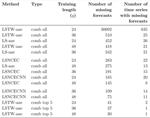
Table 3.2 contains information about number of missing forecasts, and time series, per

1_{The M3-Competition dataset contains only 22 non-monthly time series that are 100 observations}

(26)

method, type and training length. Type is here referred to as the scenario when all eleven univariate forecasting methods are used as input (comb all), or when top five univariate forecasting methods from the pre-screening step are used (comb top 5). The method LSTW-aae withq= 24 that utilizes all univariate forecasts as input too often fail to fit a model since more observations usually are required. The LSTW-aae method with q= 24 is therefore excluded fully from the evaluation. The method is included in the evaluation study whenq is equal to 36 or 48. A total of almost 3.2 million forecasts are included in the evaluation study.

Table 3.2: Number of forecasts missing, and number of time series with forecasts missing, in the common intersection of 30 858 ob-servations across 835 time series in Step 8 of the data generating procedure.

Method Type Training length (q) Number of missing forecasts Number of time series with missing forecasts

LSTW-aae comb all 24 30692 835

LS-aae comb all 24 452 26

LSNCEC comb all 24 283 22

LSNCECNN comb all 24 185 20

LSTW-aae comb top 5 24 41 2

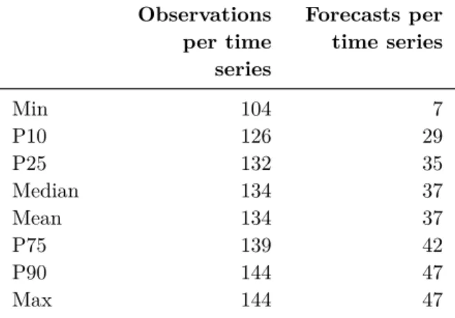
Descriptive statistics about number of observations per time series and number of forecasts per time series in the evaluation dataset is available in Table 3.3. Number of observations per time series varies from 104 to 144, across the 807 time series. The mean is 134 observations per time series. Of the time series, 50 percent of them contain between 132 and 139 observations. Number of forecasts per time series, from a single forecasting method included in the evaluation, varies from 7 to 47, with a mean of 37. Between 35 and 42 forecasts are computed from 50 percent of the time series.

(27)

Table 3.3: Summary statistics across the 29 892 observations from the 807 time series in the evaluation dataset. The tables shows the percentiles (starting with P or just named Median), min, max and mean related to number of observations per time series as well as for number of forecasts per time series.

Observations per time series Forecasts per time series Min 104 7 P10 126 29 P25 132 35 Median 134 37 Mean 134 37 P75 139 42 P90 144 47 Max 144 47

4 Results

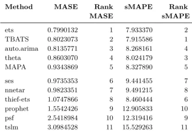
The forecasting methods described in the Methods section are applied on the M3-Competition dataset as explained in the Data section. Result from Step 4 of the data generating procedure, where the pre-screening subset with 209 time series are utilized to rank the univariate methods, is available in Table 4.1. The table contains MASE and sMAPE scores, each computed across all 17 814 observations from all 209 time series at once. This means that all observations are equally weighted but a time series with more observations has a higher impact on the measures compared to a time series with less. The table also contains a ranking for each of the two error measures; lower rank means a lower forecast error, i.e. a higher forecast accuracy. The top five forecasting methods selected, based on MASE, are ets, TBATS, auto.arima, theta and MAPA. The top five methods are the same if ranked according to sMAPE.

A complete summary of the results from Step 8 of the data generating procedure is available in Table A.1 in the appendix. It represents the evaluation across the 29 892 observations from 807 time series. Nineteen combination methods are evaluated, four without training and fifteen with training. All methods are evaluated in two scenarios, one when all eleven univariate forecasting methods are used as input and one when top five univariate forecasting methods from the pre-screening step are used.

(28)

Table 4.1: Result from evaluating univariate methods to find top 5 meth-ods based on MASE. Each method is evaluated across the same 17 814 observations from 209 time series.

Method MASE Rank

MASE sMAPE Rank sMAPE ets 0.7990132 1 7.933370 2 TBATS 0.8023073 2 7.915586 1 auto.arima 0.8135771 3 8.268161 4 theta 0.8603070 4 8.024179 3 MAPA 0.9343869 5 8.327890 5 ses 0.9735353 6 9.441455 7 nnetar 0.9823351 7 9.491215 8 thief-ets 1.0747866 8 8.460444 6 prophet 1.5542426 9 12.905833 10 psf 2.5418984 10 12.319416 9 tslm 3.0984528 11 15.529263 11

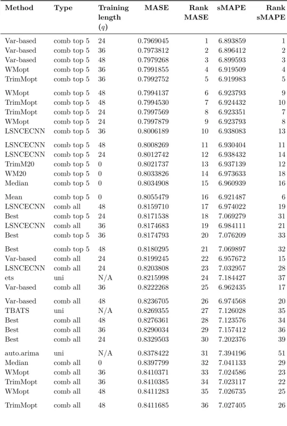
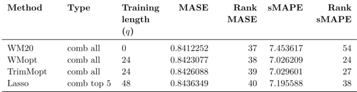
The methods requiring training are evaluated across three different training lengths except for LSTW-aae, as described in the Data section. The univariate forecasting methods are also included in the table. A total of 107 compounds are evaluated. The top 40 rows, ordered by MASE, from the table are also available in Table 4.2. Each row in the tables represents a method (for example: Var-based, LSNCECNN, median, auto.arima), type of method (if it is an univariate (uni), based on all 11 univariate methods when combined (comb all), or based on top 5 ranked univariate methods (comb top 5) from the independent pre-screening dataset) and training length (0, 24, 36 or 48 past periods for the combined methods, or written as not applicable (N/A) when it comes to the univariate methods). The columns MASE and sMAPE shows the errors from the evaluation across all observations from all time series at once; similar to what was described for Table 4.1. I.e. each row in the tables, which represents a combination of method, type and training length, is evaluated on exactly the same observations. The two ranking columns should here be interpreted similar to what was done with the previously mentioned Table 4.1.

The top 23 rows in Table 4.2 all come from methods that combine forecasts. The best MASE ranked univariate forecasting method, ets, is in 24th _{place. The differences in}

MASE score between the best combination method and the best univariate method is 0.02469. The corresponding difference for sMAPE is 0.2321 percent; here the TBATS method replace ets as the best univariate method. The result of the evaluation indicates that it is possible to combine forecasts in order to obtain a lower forecast error compared to just selecting the best univariate method.

(29)

Table 4.2: Evaluation result across the 29 892 observations from 807 time series. Shown for top 40 methods sorted on MASE.

Method Type Training length (q) MASE Rank MASE sMAPE Rank sMAPE

Var-based comb top 5 24 0.7969045 1 6.893859 1

WMopt comb top 5 36 0.7991855 4 6.919509 4

TrimMopt comb top 5 36 0.7992752 5 6.919983 5

WMopt comb top 5 48 0.7994137 6 6.923793 9

WMopt comb top 5 24 0.7997879 9 6.923793 8

LSNCECNN comb top 5 36 0.8006189 10 6.938083 13

TrimM20 comb top 5 0 0.8021737 13 6.937139 12

WM20 comb top 5 0 0.8033826 14 6.973633 18

Median comb top 5 0 0.8034908 15 6.960939 16

Mean comb top 5 0 0.8055479 16 6.921487 6

LSNCECNN comb all 48 0.8159710 17 6.974022 19

Best comb top 5 24 0.8171538 18 7.069279 31

Best comb top 5 36 0.8174793 20 7.076209 33

Best comb top 5 48 0.8180295 21 7.069897 32

Var-based comb all 24 0.8199245 22 6.957672 15

ets uni N/A 0.8215998 24 7.184427 37

TBATS uni N/A 0.8269355 27 7.126028 35

Best comb all 48 0.8276361 28 7.123576 34

Best comb all 36 0.8290034 29 7.157412 36

Best comb all 24 0.8329503 30 7.202376 39

auto.arima uni N/A 0.8378422 31 7.394196 51

Median comb all 0 0.8397799 32 7.041133 29

WMopt comb all 36 0.8410371 33 7.024586 23

TrimMopt comb all 36 0.8410385 34 7.023117 22

WMopt comb all 48 0.8411283 35 7.026735 25

(30)

Table 4.2: Evaluation result across the 29 892 observations from 807 time series. Shown for top 40 methods sorted on MASE.(continued)

Method Type Training length (q) MASE Rank MASE sMAPE Rank sMAPE WM20 comb all 0 0.8412252 37 7.453617 54

WMopt comb all 24 0.8423077 38 7.026209 24

TrimMopt comb all 24 0.8426088 39 7.029601 27

Lasso comb top 5 48 0.8436349 40 7.195588 38

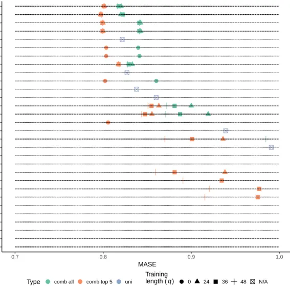
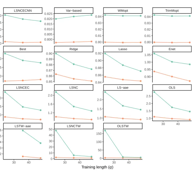
A clear pattern is visible when the scenario where all eleven methods are selected and combined is compared with the scenario where only the top five univariate methods, from the pre-screening step, are selected and combined. This is more easily seen in Figure 4.1, which is just a visualization of the information from Table A.1. The methods are listed on the y-axis while the MASE score is spread on the x-axis. Only MASE scores in the range from 0.7 up until and including 1 are included in the figure to make it easier to spot differences between the top methods. An additional version of Figure 4.1 is available in Figure A.1 in the appendix in which only observations with a MASE>3 are removed. The scores from the combination methods are seen in turquoise and (salmon) red. Red color represents the scenario when forecasts from the top five univariate methods are combined while turquoise represents when all eleven available methods are combined. The univariate forecasting methods are also available in blue. The shapes represents the training length. It is clear from the figure that the red shapes on each horizontal line in general have lower MASE score compared to the corresponding turquoise shapes. This clearly indicates adding a pre-screening process initially will increase the forecast accuracy. It should be noted that the ranking of the univariate methods, based on the 209 time series from Step 4 described in the Data section, is identical to the ranking of the univariate methods in the evaluation of the 807 time series. If a discrepancy between the two rankings occurred the result might be different. The appendix also contains Figure A.2 which is similar to Figure 4.1 but is showing the sMAPE score instead of MASE. Observations with a sMAPE score in the range from 6.8 up until and including 10 percent are seen in the figure. A zoomed out version of Figure A.2 is available in Figure A.3. Only observations with sMAPE >25 are removed in this figure.

When the top five univariate methods are used as input, then nine different methods to combine forecasts all show a better MASE score on all computed scenarios compared to the best performing univariate method, which is the ets forecast. The best performing method, utilizing top five only, seems to be the Var-based method, followed by WMopt,

(31)

OLSTW LSNCTW tslm LSTW−aae psf prophet OLS LS−aae LSNC LSNCEC thief−ets nnetar ses Enet MAPA Mean Lasso Ridge theta auto.arima TrimM20 TBATS Best WM20 Median ets TrimMopt WMopt Var−based LSNCECNN 0.7 0.8 0.9 1.0 MASE Method

Type comb all comb top 5 uni

Training

length ( q) 0 24 36 48 N/A

Figure 4.1: MASE computed for each method, type and training length when applicable. Based on the evaluation dataset with 29 892 observations from 807 time series. Shows only observations in the figure with MASE in the range from 0.7 up until and including 1.

(32)

TrimMopt and LSNCECNN. All of them are using training data. The four methods that do not use training data seems to be placed right after these. Even the so called Best method is better than the best performing univariate method. This result is easiest seen in Table 4.2 on rows 1 to 24, or via Figure 4.1. The result is similar on sMAPE.

The result from the study also shows that it is possible to create a combined forecast based on all eleven univariate methods that performs better than the best univariate method. However, the result shows that it is only possible to achieve this feat with LSNCECNN, nonetheless independently if the training length is 24, 36 or 48 periods long. The Var-based method is achieving similar, sometimes better and sometimes worse, than the best univariate method. The third best method is the Best method which manage to place somewhere between the second and third best univariate methods. It should be noted that sMAPE is more forgiving than MASE since sMAPE places six combination methods as better than the best univariate method while MASE only places one. The training based versions of the trimmed mean and winsorized mean, i.e. WMopt and TrimMopt, are among these six methods together with Median and TrimM20. The latter two are methods that do not use training data. Worth noting, the Mean method perform much worse when all eleven methods are used as input, and this effect is likely related to one or more of the worst performing univariate forecasting methods since this or they pulls up the error quite much.

All but one of the regression based approaches to combine forecasts perform rather poor. The sole exception is the mentioned LSNCECNN method. The approaches that includes time-varying weights are particular bad. Adding an auto ARIMA error term to the regression model usually does not contribute to an improvement. This might be expected since the relative short training length, between two and four times the potential seasonal length, makes it difficult to catch a pattern. A rather clear picture is available when it comes to the unbiased regression models. The more restrictive a model is, the higher the accuracy is. LSNCECNN is the most restrictive model and performs best. The second most restrictive model, LSNCEC, performs second best, while LSNC usually is in third place and the least restrictive model, OLS, is in last place.

Ridge, Lasso and Enet, i.e. the biased regression based forecast methods, generally performs better than the unbiased regression methods OLS, LSNC and LSNCEC. A similar pattern regarding restrictiveness, but in a different way, is also visible. The more restrictive Ridge and Lasso methods performs better compared to Enet. A Ridge or a Lasso method is available for selection within the Enet but they might not be chosen. The Enet’s suboptimal forecast performance might be related to overfitting in the training stage.