Graphical and Database Analysis of New Sequence of Functions Involving the Bessel Function with MatLab Implementation

(1)

Graphical and Database Analysis of New

Sequence of Functions Involving the Bessel

Function with MatLab Implementation

Jaspreet Kaur

Department of Computer Science Baba Farid Group of Institutions

Bathinda-151001, India

Ranbir Kaur Brar

Department of Computer Science Baba Farid Group of Institutions

Bathinda-151001, India

Mehar Chand

Department of Mathematics Malwa college of IT and

Managment Bathinda-151001, India

Kanwarjit Singh

Department of Computer Science T.P.D. Malwa College

Rampura Phul Bathinda-151103, India

ABSTRACT

The aim of the present paper is an attempt to introduce a new sequence of functions



, 







; , , / 0,1, 2,...

  _

n

V x a k s n , which

involving the Bessel function of first kind J

 

x . By using operational technique, some interesting generating relations and summation formulas are obtained in sections 2 and 3. The remarkable thing of this paper is the crucial MATLAB coding of the new sequence of functions, Database and Graph established using the MATLAB (R2012a) in the section (5) and (6) for different values of parameters and n=1, 2, 3 and 4. The reader can establish Database and Graph using the same program for any value of n.

General Terms

Special function, Sequence of Function, Matlab.

Keywords

Special Function, Generating function, Bessel function of first kind, Sequence of function, Matlab.

1. INTRODUCTION

In the present Era, MATLAB is a high-performance language for technical computing. It integrates computation, visualization, and programming in an easy-to-use environment where problems and solutions are expressed in familiar mathematical notation. Typical uses include:

 Math and computation

 Algorithm development

 Modeling, simulation, and prototyping

 Data analysis, exploration, and visualization

 Scientific and engineering graphics

 Application development, including Graphical User Interface building

In pure mathematics, since Matlab is an integrated computer software which has three functions: symbolic computing, numerical computing and graphics drawing. Matlab is capable to carry out many functions including computing polynomials and rational polynomials, solving equations and computing many kind of mathematical expressions. One can also use Matlab to calculate the limit, derivative, integral and Taylor

series of some mathematical expressions. With Matlab, The graphs of functions with one or two variables can be easily drawn in selected domain. Therefore, functions can be studied by visualization for their main Characteristics. Matlab is also a system which can be easily expanded. Matlab provides many powerful software packages which can be easily incorporated into the clients system. Recently, there are many papers in the literature which are devoted to the application of Matlab in mathematical analysis, see the work of Stephen [22], Dunn [6], Shampine and Robert [16].

The distinct scientific communities that are working on various aspects of automatic analysis of data include Combinatorial Pattern Matching, Data Mining, Computational Statistics, Network Analysis, Text Mining, Image Processing, Syntactical Pattern Recognition, Machine Learning, Statistical Pattern Recognition, Computer Vision, and many others. Bessel functions are a series of solutions to a second order differential equation that arise in many diverse situations. While special types of what would later be known as Bessel functions were studied by Euler, Lagrange, and the Bernoullis, the Bessel functions were first used by F. W. Bessel to describe three body motion, with the Bessel functions appearing in the series expansion on planetary perturbation [8]. The subject of Bessel Functions and applications is a very rich subject; nevertheless, due to space and time restrictions and in the interest of studying applications. Appropriate development of zeroes, modified Bessel functions, and the application of boundary conditions can be studied in the work of Jennifer Niedziela [9].

(2)

   





2 2 0 1 ( )

2 ! 1

   _         



k k k

k

x J x

k k (1.1)

Operational techniques have drawn the attention of several researchers in the study of sequences of functions and polynomials.

In 1956, Chak [1] defined a class of polynomials as:

 

_{ }

 

,

 _    _   _

 

n kn n x k x n k

G x x e x D x e (1.2)

Where k is constant and n0,1, 2,...,D d.

dx

Gould and Hopper [7] introduced generalized Hermite polynomials in 1962 as:





 





, ,

1  exp  exp 

  _  _

r n

n a r n a r

H x a p

x px D x px (1.3)

Chatterjea [4] studied as a class of polynomials for generalized Laguerre polynomials in 1964:

 

_

_

  





1 2 1

, 1 exp exp !              rn n

n r r

T x p

x px x D x px

n

(1.4)

In 1968, Singh [17] studied the generalized Truesdell polynomials defined as:

 

_

_

 





, , exp exp     _ _  _  _ n n r r

T x r p

x px xD x px

(1.5)

Srivastava and Singh [19] introduced a general class of polynomials in 1971 as:

 

_

_

 

1







, , , 1 exp exp !             n n

kn r k r

G x r p k

x px x D x px

n

(1.6)

In 1971, the Rodrigues formula for generalized Lagurre polynomials is given by Mittal [11] as:

 

_{ }

 







 



1 exp exp !     _  _  _  _ kn n n k k T x

x p x D x p x

n

(1.7)

Where p xk

 

is a polynomial in x of degree k. Mittal [12] also proved following relation for (1.7) as:

 

_{ }

 







 



1 1 exp exp !        _ _  _  _ s kn n n

k s k

T x

x p x T x p x

n

(1.8)

Where s is constant and Tsx s



xD



.

Recently, Shukla and Prajapati [21] obtained several propertie of (7) .

Chandel [2] also studied a class of polynomials defined in 1973 as:





  





, , , exp exp     _ _  _  _ k n n

r k r

T x r p

x px x D x px

(1.9)

In 1974, Chandel [3] established a generalization of polynomial system as:

 





 

, ,  hg x k n_ hg x_

n

G h g x k e x D e (1.10)

Where g x

 

is a function of ,x h and k are constants. In the same year, Srivastava [20] discussed some operational formulas generalized function Fnr m, 



x a k p, , ,



in following the form:  

_

_

  





, , , , exp exp  _  _  _  _ r m n n

a r k a km r

F x a k p

x px x D x px

(1.11)

In 1975, Joshi and Parjapat [10] introduced the a class of polynomial:  

_

_

 









 





, , exp ! exp            _  _      n nk _n k

M x a k

x

p x x a xD

n

x p x

(1.12)

Subsequently in 1975, Patil and Thakare [14] have obtained several formulae and generating relation for:

 

_

_

 









, , , , , exp exp       _ _ _  _  _  _{ }  _ n n

r k sn r

P x r s a k

x px x xD x px

(1.13)

In 1979, Srivastava and Singh [18] studied a sequence of functions Vn 



x a k s; , ,



defined as:

 

_

_

 







 



; , , exp exp !         _  _ n n k k

V x a k s x

p x x p x

n

(1.14)

By employing the operator xa



sxD



, where s is constant and p xk

 

is a polynomial in x of degree k . A new sequence of function



V_n , 



x a k s; , ,



/n0,1, 2,...



is introduced in this paper as:

 

_

_

 





 



 



, , ; , , 1 !        _ _  _  _ n n a s

k x k

V x a k s

x J p x T x J p x

n

(3)

Where ,





,

  

a s a x

d

T x s xD D

dx, a and s are constants,

0

 , k is finite and non-negative integer, p x_k

 

is a polynomial in x of degree k and J

 

x is a Bessel function of first kind defined in equation (1.1).

Some generating relations and finite summation formulae of class of polynomials or sequence of function have been obtained by using the properties of the differential operators.









, ,1

, 1

   

a s a a a

x x

T x s xD T x xD , where D d

dx, is based

on the work of Mittal [13], Patil and Thakare [14], Srivastava and Singh[18].

Some useful Operational Techniques are given below:







 











, 1/ exp 1 1    _  _     a s x s a

a _a a

tT x f x

x ax t f x ax t

(1.16)







 











, 1 1/ exp 1 1         _ _   

a s an x

s

a a

tT x f x

x at f x at

(1.17)

 

, , ,1 0  _     _{ }  



n a s x

n m m

a s a

x x

m

T xuv

n

x T v T u

m

(1.18)









 



1

1 1 1 2

1 3 ... 1 ( 1) 

                 _{ }   m m

xD a xD a xD

a xD m a xD x

a x a (1.19)









 

0 1 1 !    _{ }          _ _  



m a a m m at at at a m (1.20)

2. GENERATING RELATIONS

 

_

_







 















, 0 1/ ; , , 1 1            _ _     



an n

n n s a k a k

V x a k s x t

at J p x

J p x at

(2.1)  

_

_







 















, 0 1 1/ ; , , 1 1              _ _    



an an n

n n s a k a k

V x a k s x t

at J p x

J p x at

(2.2)  

_

_







 















 



_

_



, 0 1/ 1/ , ; , , 1 1

1 ; , ,

            _ _             



n n n s k a a k a n m n

V x a k s t m

J p x

at

J p x at

V x at a k s

(2.3)

Proof of (2.1):

From (1.15), we consider

 

_

_









, 0 , ; , ,

( ) exp( ) ( )

              



n n n a s

k x k

V x a k s t

x J p x tT x J p x

(2.4)

Using operational technique (1.16), above equation (2.4) reduces to:  

_

_









, 0 1/ ; , ,

( ) (1 ) (1 )

                     



n n n s

a a a a

k k

V x a k s t

x J p x x ax t J p x ax t







1/



(1 ) ( ) (1 )

      _ _ _     s

a a a a

k k

ax t J p x J p x ax t

(2.5) And replacing t by txa, this gives (2.1).

Proof of (23):

Again from (1.15), we have

 

_

_









, 0 , ; , ,

( ) exp( ) ( )

           _  _  _  _



an an n

n n

a s an

k x k

x V x a k s t

x J p x tT x J p x

(2.6)

applying the operational technique (1.17), we get

 

_

_



 



















, 0 1 1/ 1 1/ ; , ,

( ) 1 1

1 ( ) 1

              _  _     __  __     __  __



an an n

n n s a a k k s a a k k

x V x a k s t

x J p x x at J p x at

at J p x J p x at

(2.7)

This proves (2.2).

Proof of (2.3):

We can write (1.15) as,

 

  , , ( ( )) 1 ! ( ; , , ) ( ( ))           n a s x k v n k

T x J p x

n x V x a k s

J p x (2.8)

(4)

 







 







  , , , ,

exp ( ( ))

1

!exp ( ; , , )

( ( ))              _ _   n a s a s

x x k

v a

x n

k

t T T x J p x

n tT x V x a k s

J p x

 

  , 0 , , ( ( )) ! 1

!exp ( ; , , )

( ( ))      _          _ _  



m _{a s} m n

x k m v a s x n k t

T x J p x

m

n T x V x a k s

J p x (2.9)

Using the operational technique (1.16), above equation can be written as

 

















 





, 0 1/ 1/ , ( ( )) ! 1 ! 1 1

1 ; , ,

       _     _ _           



m m n a s x k m s a _a a a k a v a n t

T x J p x

m

n x ax t

J p x ax t

V x ax t a k s

(2.10) use of (2.8) gives





 

_

_





 













, 0 1/ , 1/ ! 1 ; , , ! ! ( ( ))

1 ; , ,

1 1               _ _       _     



m v

m n m k a v a s _n a a a a k

t m n

x V x a k s

m n J p x

V x ax t a k s

x ax t

J p x ax t

(2.11) Therefore  

_

_

















 





, 0 1/ 1/ , ; , , ( ( )) 1 1

1 ; , ,

           _ _             



v m

m n m

s

a a k

a a k a v a n m n

V x a k s t n

J p x

ax t

J p x ax t

V x ax t a k s

(2.12) And replacing t by txa, this gives the result (2.3).

3. FINITE SUMMATION FORMULAE

 

_

_

 

_

_

, ,0 0 ; , , 1 ; , , !           _{ }  



n m a n m m m

V x a k s

ax V x a k s

m a (3.1)

 

_

_

 

_

_

, , 0 ; , , 1 ; , , !              _ _  



n m a n m m m

V x a k s

ax V x a k s

m a (3.2)

Proof of the (3.1) equation:

From equation (1.15), We have:

 

_

_

 





 

_

_{ }

_

, , 1 ; , , 1 !        _  _  _  _ n n a s

k x k

V x a k s

x J p x T xx J p x

n (3.3)

Using the operational technique (1.18), we have:

 

_

_

 





 

_

_{ }

_

   

,

, ,1 1

0 ; , , 1 !             _ _  _{ } _  _  



n

n _{a s} n m _a m

k x k x

m

V x a k s

n

x J p x x T J p x T x

m n

 





_

_

 

















 

















 

0 1 1 ! ! ! ! 2 ... 1

1 1 1 2 ...

1 1                          _{ }  _             _



n

a n m k

m

am k

n

x J p x x x

n m n m

s xD s a xD s a xD

s n m a xD J p x x

xD a xD a xD

m a xD x

 





_

_







 



0 1 0 1 ! !                _  _ _{ }  





n an k m n m m k i m

J p x x

m n m

s ia xD J p x a

a (3.4)

Put 0 and replacing n by nm in (3.3), we get:

 

_

_







 



 



 



,0 , ; , , 1 !         _  _  n m n m a s

k x k

V x a k s

J p x T J p x

n m





 



 



 





 





, ,0 1 ! 1 ; , ,         _  _   n m a s x k n m k

T J p x

n m

V x a k s

J p x (3.5)

This gives











 



 





 





1 0 ,0 1 ! 1 ; , ,             _  _  



n m k i

a m n

n m k

s ia xD J p x

n m

x V x a k s

J p x (3.6)

From equation (3.4) and (3.6) we have the main the result Proof the equation (3.2):

Equation (1.15) can be written as:

 

_

_

 





 

_

_{ }

_

, 0 , ; , , exp          _ _  _  _



n n n a s

k x k

V x a k s t

x J p x T x J p x (3.7)

Applying the (1.16) in equation (3.1), we have:

 

_

_

 













, 0 1/ ; , , 1 1                 _ _    



n n n s a

a _a a

k k

V x a k s t

x J p x x ax t J p x ax t







 







1/



1 1       _ _ 

  _a s   _a a

a

k k

ax t J p x J p x ax t

(5)

Applying the result from equation (1.20); equation (3.8) reduces to:





 









0 1/ 1 ! 1          _ _        _ _    



m a s a _a m m a a k k ax t ax t a m

J p x J p x ax t

 

_

_{ }

_

 



 



0 , ! exp              _ _       



m a k m m a s x k ax t

x J p x

a m

T x J p x

 





 



 



0 0 , ! !                 _ _       



m a n m

m n m

n a s

k x k

ax t x

a m n

J p x T x J p x

 





 





 



 



0 0 , ! !                _ _        



m a n n

n m m

n m a s

k x k

ax t x

a m n m

J p x T x J p x

(3.9) Now equating the coefficient of tn , we get

 

_

_

 





 





 



 



, 0 , ; , , ! !                _ _        



n m a n m m n m a s

k x k

V x a k s

ax x

a m n m

J p x T x J p x _(3.10)

Using the equation (1.15) in (3.10) we have the result (3.2)

4. SPECIAL CASES

The interesting special cases/relationships between (1.15) and class of polynomials (1.2)-(1.14) can also be obtained for appropriate values of alpha, nu, a, k and s.

The, Matlab is one of the important aspect mainly in the field of sciences and engineering, Therefore, the imperative Matlab coding established for each parameter of equation (1.15) and some interesting database and graphs also established in the section 5. Using this coding reader may obtain large number of graphs of equation (1.15), which gives the eccentric characteristics in the area of sequence of functions or class of polynomials

5. PROGRAMMING OF THE NEW

SEQUENCE

OF

FUNCTIONS

IN

MATLAB

Code of New sequence of functions:

function [Vn] = gnsbj2(alpha,nu,a,k,s,x)

%Graph of Vn(alpha,nu,a,k,s,x) %P=Pn(alpha,nu,a,k,s,x)=(1/n!)*x^-alpha*besselj(nu,x^k)*Tn^(a,s)

%(x^a*(s+x*D)(x^alpha)*besselj(nu,-x^k)), where n=1,2,3,…

syms x

%n=input('please enter n:');

n=2;

E1= besselj(nu,-x.^k); y=(x.^alpha).*E1; for i=1:n

y=(x.^a).*(s.*y+x.*diff(y)); end E2=besselj(nu,x.^k); v=(1./factorial(n)).*(1./(x.^alpha)).*E2.*y; %Vn=subs(v,x,-.5:.1:.5); Vn=subs(v,x); end

Plot The Graph: Command window: hold on

V1= ezplot(gnsbj1(1,1,1,1,1,x),[-2:.5:2]); V2= ezplot(gnsbj2(1,1,1,1,1,x),[-2:.5:2]); V3= ezplot(gnsbj3(1,1,1,1,1,x),[-2:.5:2]); V4= ezplot(gnsbj4(1,1,1,1,1,x),[-2:.5:2]); title('Vn(alpha,nu,a,k,s,x);n=1,2,3,4') hold off

set(V1,'color','r') set(V2,'color','b') set(V3,'color','g') set(V4,'color','m')

legend('V1(1,1,1,1,1,x)','V2(1,1,1,1,1,x)','V3(1,1,1,1,1,x)','V4( 1,1,1,1,1,x)')

6. DIFFERENT

DATABASES

AND

GRAPHS USING MATLAB

The new sequence



, 







; , , / 0,1, 2,...

  _

n

V x a k s n introduced

in equation (1.15), takes place in the form of Vn(alpha,nu,a, k,s,x) to establish Database and Graph for different values of parameters alpha, nu, a, k, s and (n = 0, 1, 2, 3,…). Four different Database for different values of parameters for n=1,2,3 in the interval

  

2 x

2

with difference .5 and

0.5

0.5 

 

x

with difference 0.1 are established, as shown in Data base in table 1, 2, 3, 4 & 5 and their corresponding

Graphs are plotted.

[image:5.595.76.521.699.764.2]

(6.1) First Database and Graph:

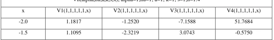
Table 1. Database of sequence of function Vn(1,1,1,1,1,x) for n=1:4 Vn(alpha,nu,a,k,s,x); alpha=1;nu=1; a=1; k=1; s=1;n=1:4

x V1(1,1,1,1,1,x) V2(1,1,1,1,1,x) V3(1,1,1,1,1,x) V4(1,1,1,1,1,x)

-2.0 1.1817 -1.2520 -7.1588 51.7684

(6)

-1.0 0.5304 -0.9386 1.3300 -1.6043

-0.5 0.0862 -0.0839 0.0676 -0.0488

0 0 0 0 0

0.5 -0.0862 -0.0839 -0.0676 -0.0488

1.0 -0.5304 -0.9386 -1.3300 -1.6043

1.5 -1.1095 -2.3219 -3.0743 -0.5750

2.0 -1.1817 -1.2520 7.1588 51.7684

Fig. 1 Based on table (1)

[image:6.595.85.516.196.583.2]

(6.2) Second Database and Graph:

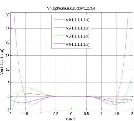
Table 2. Database of sequence of function Vn(-1,2,1,2,1) for n=1:4 Vn(alpha,nu,a,k,s,x); alpha=-1;nu=2; a=1; k=2; s=1;n=1:4

x V1(-1,2,1,2,1,x) V2(-1,2,1,2,1,x) V3(-1,2,1,2,1,x) V4(-1,2,1,2,1,x)

-2.0 1.4455 -14.1741 26.3861 313.2720

-1.5 -0.5153 -0.3966 9.0717 -42.1274

-1.0 -0.0483 0.1034 -0.1567 0.1564

-0.5 -0.0001 0.0001 -0.0001 0.0001

0 0 0 0 0

-2

-1.5

-1

-0.5

0

0.5

1

1.5

2 -5

0

5

10

15

20

25

30 x-axis

Vn(alpha,nu,a,k,s,x);n=1,2,3,4

V

n

(1

,1

,x

)

V1(1,1,1,1,1,x)

V2(1,1,1,1,1,x)

V3(1,1,1,1,1,x)

[image:6.595.84.513.645.759.2]

(7)

0.5 0.0001 0.0001 0.0001 0.0001

1.0 0.0483 0.1034 0.1567 0.1564

1.5 0.5153 -0.3966 -9.0717 -42.1274

2.0 -1.4455 -14.1741 -26.3861 313.2720

[image:7.595.76.510.128.524.2]

(6.3) Third Database and Graph:

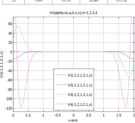
Table 3. Database of sequence of function V1 for different values of parameters Vn(alpha,nu,a,k,s,x); alpha=2,4,6;nu=2; a=3; k=2; s=1;n=1

x V1(2,2,3,2,1,x) V1(4,2,3,2,1,x) V1(6,2,3,2,1,x) V1(8,2,3,2,1,x)

-2.0 2.5998 0.4784 -1.6431 -3.7645

-1.5 -2.8178 -3.9233 -5.0288 -6.1343

-1.0 -0.0879 -0.1143 -0.1407 -0.1671

-0.5 -0.0001 -0.0001 -0.0001 -0.0001

0 0 0 0 0

0.5 0.0001 0.0001 0.0001 0.0001

1.0 0.0879 0.1143 0.1407 0.1671

1.5 2.8178 3.9233 5.0288 6.1343

2.0 -2.5998 -0.4784 1.6431 3.7645

-2

-1.5

-1

-0.5

0

0.5

1

1.5

2 -120

-100

-80

-60

-40

-20

0

20

40

60 x-axis

Vn(alpha,nu,a,k,s,x);n=1,2,3,4

V

n

(-1

,2

,1

,2

,1

,x

)

V1(-1,2,1,2,1,x)

V2(-1,2,1,2,1,x)

V3(-1,2,1,2,1,x)

[image:7.595.84.515.594.770.2]

(8)

[image:8.595.83.515.80.461.2]

(6.4) Fourth Database and Graph:

Table 4. Database of sequence of function V2 for different values of parameters Vn(alpha,nu,a,k,s,x); alpha=2,4,6,8;nu=2; a=3; k=2; s=1;n=2

x V2(2,2,3,2,1,x) V2(4,2,3,2,1,x) V2(6,2,3,2,1,x) V2(8,2,3,2,1,x)

-2.0 -335.4357 -334.6040 -299.8294 -231.1119

-1.5 30.4355 58.7832 94.5931 137.8653

-1.0 0.4155 0.6573 0.9520 1.2995

-0.5 0.0000 0.0001 0.0001 0.0001

0 0 0 0 0

0.5 0.0000 0.0001 0.0001 0.0001

1.0 0.4155 0.6573 0.9520 1.2995

1.5 30.4355 58.7832 94.5931 137.8653

2.0 -335.4357 -334.6040 -299.8294 -231.1119

-2

-1.5

-1

-0.5

0

0.5

1

1.5

2 -10

-5

0

5

10 x-axis

Vn(alpha,nu,a,k,s,x);n=1

V

n

(a

lp

h

a

,2

,3

,2

,1

,x

),

a

lp

h

a

=

2 ,4

,6

,8

V1(2,2,3,2,1,x)

V1(4,2,3,2,1,x)

V1(6,2,3,2,1,x)

[image:8.595.73.524.531.715.2]

(9)

[image:9.595.76.512.79.450.2]

(6.5) Fifth Database and Graph:

Table 5. Database of sequence of function V2 for different values of parameters Vn(alpha,nu,a,k,s,x); alpha=nu=1; a=2:5; k=3:6; s=4:7;n=2

x V2(1,1,2,3,4,x) V2(1,1,3,4,5,x) V2(1,1,4,5,6,x) V2(1,1,5,6,7,x)

-0.5 -0.0097 -0.9899x10-3 -0.9151x10-4 -0.7926x10-5

-0.4 -0.0010 -0.0436 x10-3 _{-0.0165 x10}-4 _{-0.0058 x10}-5

-0.3 -0.0001 -0.0008 x10-3 -0.0001 x10-4 -0.0000 x10-5

-0.2 -0.0000 -0.0000 x10-3 -0.0000 x10-4 -0.0000 x10-5

-0.1 -0.0000 -0.0000 x10-3 _{-0.0000 x10}-4 _{-0.0000 x10}-5

0 0 0 0 0

0.1 -0.0000 -0.0000 x10-3 -0.0000 x10-4 -0.0000 x10-5

0.2 -0.0000 -0.0000 x10-3 -0.0000 x10-4 -0.0000 x10-5

0.3 -0.0001 -0.0008 x10-3 -0.0001 x10-4 -0.0000 x10-5

0.4 -0.0010 -0.0436 x10-3 -0.0165 x10-4 -0.0058 x10-5

0.5 -0.0097 -0.9899 x10-3 _{-0.9151 x10}-4 _{-0.7926 x10}-5

-2

-1.5

-1

-0.5

0

0.5

1

1.5

2 -200

-150

-100

-50

0

50

100

150

200

250

300 x-axis

Vn(alpha,nu,a,k,s,x);n=2

V

2 (a

lp

h

a

,2

,3

,2

,1

,x

),

a

lp

h

a

=

2 ,4

,6

,8

V2(2,2,3,2,1,x)

V2(4,2,3,2,1,x)

V2(6,2,3,2,1,x)

[image:9.595.83.515.508.711.2]

(10)

(6.6) Different Graphs Of The Sequence Of Functions For Different Range

Fig. 6 Graphs of the sequence for the intervals [-0.5, 0.5] and [-1, 1] for n=1

-0.5

-0.4

-0.3

-0.2

-0.1

0

0.1

0.2

0.3

0.4

0.5 -9

-8

-7

-6

-5

-4

-3

-2

-1

0 x 10

-7

x-axis

Vn(alpha,nu,a,k,s,x);n=2

V

2 (1

,1

,a

,k

,s

,x

)

V2(1,1,2,3,4,x)

V2(1,1,3,4,5,x)

V2(1,1,4,5,6,x)

V2(1,1,5,6,7,x)

-0.5 -0.4 -0.3 -0.2 -0.1 0 0.1 0.2 0.3 0.4 0.5

-5 0 5

x 10-6 V1(2,2,3,2,1,x)

-1 -0.8 -0.6 -0.4 -0.2 0 0.2 0.4 0.6 0.8 1

-0.01 -0.005 0 0.005 0.01

[image:10.595.88.527.78.448.2] [image:10.595.106.485.469.735.2]

(11)

Fig. 7 Graphs of the sequence for the intervals [-3, 3] and [-5, 5] for n=1

Fig. 8 Graphs of the sequence for the intervals [-0.5, 0.5] and [-1, 1] for n=2

-3 -2 -1 0 1 2 3

-10 -5 0 5 10

V1(2,2,3,2,1,x)

-5 -4 -3 -2 -1 0 1 2 3 4 5

-50 0 50

V1(2,2,3,2,1,x)

-0.5 -0.4 -0.3 -0.2 -0.1 0 0.1 0.2 0.3 0.4 0.5

-3 -2 -1 0

x 10-4 V2(1,1,a,k,s,x)

V2(1,1,2,3,4,x) V2(1,1,3,4,5,x)

-1 -0.8 -0.6 -0.4 -0.2 0 0.2 0.4 0.6 0.8 1

-4 -3 -2 -1 0

V2(1,1,a,k,s,x)

[image:11.595.123.477.78.346.2] [image:11.595.127.478.390.640.2]

(12)

[image:12.595.124.480.82.353.2]

Fig. 9 Graphs of the sequence for the intervals [-2, 2] and [-3, 3] for n=1

Fig. 10 Graphs of the sequence for the intervals [-1,1] and [-3,3] for n=1

-2 -1.5 -1 -0.5 0 0.5 1 1.5 2

-5 0 5

V1(1,1,a,k,s,x)

V1(1,1,2,3,4,x) V1(1,1,3,4,5,x)

-3 -2 -1 0 1 2 3

-20 -10 0 10 20

V1(1,1,a,k,s,x)

V1(1,1,2,3,4,x) V1(1,1,3,4,5,x)

-1 -0.5 0 0.5 1

-2 -1.5 -1 -0.5 0

V1(alpha,nu,2,3,2,x)

V1(2,1,2,3,2,x) V1(4,1,2,3,2,x) V1(6,1,2,3,2,x) V1(8,1,2,3,2,x)

-3 -2 -1 0 1 2 3

-10 -5 0 5

V1(alpha,nu,2,3,2,x)

[image:12.595.105.492.404.676.2]

(13)

[image:13.595.113.488.91.341.2]

Fig. 11 Graphs of the sequence for the intervals [0, 2] and [0, 4] for n=1

7. INTERPRETATION OF THE ABOVE

DATABASE AND GRAPHS

The different values of the parameters, as assigned for equation (1.15) are taken to establish different databases and their graphs. In this section interpretation of the above database and graphs are made for different parameters of the new sequence of functions.

(I) The first database and graph of the sequence of functions Vn(1,1,1,1,1,x) for n=1, 2, 3 and 4 are established for the range

  

2 x

2.

From the database (1) and Figure (1), it is easily observed that V1(1,1,1,1,1,x) and V3(1,1,1,1,1,x) are anti-symmetric in the interval about the line x=0 whereas V2(1,1,1,1,1,x) and V4(1,1,1,1,1,x) are symmetric about the line x=0 for the given interval.

(II) The second database and graph of the sequence of functions Vn(-1,2,1,2,1,x) for n=1, 2, 3 and 4 are established for the range

  

2 x

2.

From the database (2) and Figure (2), it is easily observed that V1(-1,2,1,2,1,x) and V3(-V1(-1,2,1,2,1,x) are anti-symmetric in the interval about the line x=0 whereas V2(-1,2,1,2,1,x) and V4(-1,2,1,2,1,x) are symmetric about the line x=0 for the given interval.

(III)The third database and graph of the sequence of functions V1(alpha,2,3,2,1,x) for alpha=2, 4, 6, 8 are established for the range

  

2 x

2.

From the database (3) and Figure (3), it is easily observed that V1(2,2,3,2,1,x), V1(4,2,3,2,1,x), V1(6, 2,3,2,1,x) and

V1(8,2,3,2,1,x) are anti-symmetric about the line x=0 for the given interval.

(IV)The fourth database and graph of the sequence of functions V2(alpha,2,3,2,1,x) for alpha=2, 4, 6, 8 are established for the range

  

2 x

2.

From the database (4) and Figure (4), it is easily observed that V2(2,2,3,2,1,x), V2(4,2,3,2,1,x), V2(6, 2,3,2,1,x) and V2(8,2,3,2,1,x) are symmetric about the line x=0 for the given interval.

(V) The fifth database and graph of the sequence of functions V2(1,1,a,k,s,x) for different values of the parameters are established for the range



0.5  

x

0.5.

From the database (5) and Figure (5), it is easily observed that V2(1,1,2,3,4,x), V2(1,1,3,4,5,x), V2(1,1,4,5,6,x) and V2(1,1,5,6,7,x) are symmetric about the line x=0 for the given interval. The graph of the sequence for all the parameters lies below the line y=0 in the interval

0.5

0.5. 

 

x

(VI)In the figure 6 and 7 for the sequence V1(2,2,3,2,1,x), where x lies in the intervals [-0.5, 0.5], [-1,1], [-3,3] and [-5,5]; it is observed that graphs for the said range of the sequence of function are anti-symmetric. The figures 8 and 9 of the sequences V1(1,1,2,3,4,x) and V1(1,1,3,4,5,x) for the intervals [-0.5, 0.5], [-1,1], [-2,2] and [-3,3] are also anti-symmetric. Figure 10 and 11of the sequences V1(alpha,1,2,3,2,x) where alpha=2,4,6,8; for the interval [-1,1], [-3,3], [0,2] and [0,4] also can be easily interpreted.

0 0.5 1 1.5 2

-4 -2 0 2

V1(alpha,nu,2,3,2)

V1(2,1,2,3,2,x) V1(4,1,2,3,2,x) V1(6,1,2,3,2,x) V1(8,1,2,3,2,x)

0 1 2 3 4

-10 0 10

V1(alpha,nu,2,3,2)

(14)

8. CONCLUSION

This paper presents several cases of MATLAB applications in mathematical analysis including generating the graph and database of sequence of function. Program made for sequence of function is easy to establish and implementation for Graphs and Data-Bases. Authors come to the conclusion on the basis of above interpretation that the sequence of functions is either symmetric or anti-symmetric for different values of the parameters for even and odd values of n in particular. The present paper has enabled to find the values of sequence of functions for different values of parameters and have paved the way for comparison of trends.

9. REFERENCES

[1] Chak, A. M., 1956, A class of polynomials and generalization of stirling numbers, Duke J. Math., 23, 45-55.

[2] Chandel, R.C.S., 1973, A new class of polynomials, Indian J. Math., 15(1), 41-49.

[3] Chandel, R.C.S., 1974, A further note on the class of polynomials ,k



, ,



n

T x r p ,Indian J. Math., 16(1), 39-48.

[4] Chatterjea, S. K., 1964, On generalization of Laguerre polynomials, Rend. Mat. Univ. Padova, 34, 180-190. [5] Craven Thomas and Csordas George, 2006, The

Fox-Wright functions and Laguerre multiplier sequences, J. Math. Anal. and Appl. 314, 109-125.

[6] Dunn, Peter K., Understanding statistics using computer demonstrations. Journal of Computers in Mathematics and Science Teaching, 22 (3). pp. 261-281. ISSN 0731-9258, 2003.

[7] Gould, H. W. and Hopper, A. T., 1962, Operational formulas connected with two generalizations of Hermite polynomials, Duck Math. J., 29, 51-63.

[8] J. J. O' Connor and R. E. F., Friedrich Wilhelm Bessel (School of Mathematics and Statistics University of St Andrews Scotland, 1997).

[9] Jennifer Niedziela, Bessel Functions and Their Applications, University of Tennessee-Knoxville, (Dated: October 29, 2008).

[10]Joshi, C. M. and Prajapat, M. L., 1975, The operator

T

_{a k}_,

, and a generalization of certain classical polynomials, Kyungpook Math. J., 15, 191-199.

[11]Mittal, H. B., 1971, A generalization of Laguerre polynomial, Publ. Math. Debrecen, 18, 53-58.

[12]Mittal, H. B., 1971, Operational representations for the generalized Laguerre polynomial, Glasnik Mat.Ser III, 26(6), 45-53.

[13]Mittal, H. B., 1977, Bilinear and Bilateral generating relations, American J. Math., 99, 23-45.

[14]Patil, K. R. and Thakare, N. K., 1975, Operational formulas for a function defined by a generalized Rodrigues formula-II, Sci. J. Shivaji Univ. 15, 1-10. [15]Rainville, E.D.,1971 Special functions, Chelsea

Publishing Company, Bronx, New York.

[16]Shampine，L. F., Robert Ketzscher， Using AD to solve BVPs in MATLAB Journal ACM Transactions on Mathematical Software, Volume 31 Issue 1, ACM New York, NY, USA, March 2005.

[17]Singh, R. P., 1968, On generalized Truesdell polynomials, Rivista de Mathematica, 8, 345-353. [18]Srivastava, A. N. and Singh, S. N., 1979, Some

generating relations connected with a function defined by a Generalized Rodrigues formula, Indian J. Pure Appl. Math., 10(10), 1312-1317.

[19]Srivastava, H. M. and Singhal, J. P., 1971, A class of polynomials defined by generalized Rodrigues formula, Ann. Mat. Pura Appl., 90(4), 75-85.

[20]Shrivastava, P. N., 1974, Some operational formulas and generalized generating function, The Math. Education, 8, 19-22.

[21]Shukla, A. K. and Prajapati J. C., 2007, On some properties of a class of Polynomials suggested by Mittal, Proyecciones J. Math., 26(2), 145-156.