Titanium surface modification by oxidation for biomedical application

(1)

The University of New South Wales

Faculty of Science

School of Materials Science & Engineering

Titanium Surface Modification by Oxidation for

Biomedical Application

A Thesis

by

Hasan Z. Abdullah

Submitted in Partial Fulfilment of the

Requirements for the Degree

of

Doctor of Philosophy

in

Materials Science and Engineering

(2)

ABSTRACT

Surface modification is a process that is applied to the surfaces of titanium substrates in

order to improve the biocompatibility after implanting in the body. Two methods were

used in the present work: Anodisation and gel oxidation. Anodisation was

performed at room temperature in strong mineral acids (sulphuric acid (H2SO4) and phosphoric acid (H3PO4)), an oxidising agent (hydrogen peroxide (H2O2)), mixed

solutions of the preceding three, and a weak organic acid mixture (β-glycerophosphate

+ calcium acetate). The parameters used in anodisation were: Concentrations of the

electrolytes, applied voltage, current density, and anodisation time. Gel oxidation was

carried out by soaking titanium substrates in sodium hydroxide (NaOH) aqueous

solutions at different concentrations (0.5 M, 1.0 M, 5.0 M, and 10.0 M) at 60°C for 24 h,

followed by oxidation at 400°, 600°, and 800°C for 1 h.

Conceptual models representing changes in the microstructure as a function of the

experimental parameters were developed using the anodisation data. The relevant

parameters were: Applied voltage, current density, acid concentration, and anodisation

time:

• The model for anodisation using the strong acid (H2SO4) illustrates the growth rate

of the film, identification of the threshold for the establishment of a consistent

microstructure, and prediction of the properties of the film.

• For the oxidising agent (H2O2), two models were developed: Current-control and

voltage-control, the applicability of which depends on the scale of the current

density (high or low, respectively). These models are interpreted in terms of the

coherency/incoherency of the corrosion gel, arcing, and porosity.

• The model for the strongest acid (H3PO4) is similar to that of H2O2 in

current-control mode, although this system showed the greatest intensity of arcing

and consequent pore size.

• Anodisation in mixed solutions uses Ohm’s law to explain four stages of film

growth in current-control mode. These stages describe the thickness of the gel, its

(3)

v

• Anodisation in weaker organic acids allows the most detailed examination of the

anodisation process. Both current density and voltage as a function time reveal the

nature of the process in six stages: (1) instrumental response, (2 and 3) gel

thickening, (4) transformation of the amorphous gel to amorphous titania, (5)

recrystallisation of the amorphous titania, and (6) subsurface pore generation upon

establishment of a consistent microstructure.

Gel oxidation was done at low and high NaOH concentrations followed by oxidation.

Three models were developed to represent the gel oxidation process: (1) Low

concentration, (0.5 M and 1.0 M NaOH), (2) Medium concentration (5.0 M NaOH), and

(3) high concentration (10.0 M NaOH). For the low concentrations with increasing

temperature, the model involves: (1) amorphous sodium titanate forms over a layer of

amorphous anatase and (2) a dense layer of rutile forms. For the high concentrations

with increasing temperature, the model involves: (1) amorphous sodium titanate forms

over a layer of amorphous anatase, (2) a dense layer of anatase forms and raises up the

existing porous anatase layer, and (3) the dense and porous anatase layers transform to

dense and porous rutile layers, respectively. The main difference between the two is

the retention of crystalline sodium titanate in the higher NaOH concentration.

Anodised and gel oxidised samples subsequently were soaked in simulated body fluid in

order to study the precipitation of hydroxyapatite in the absence and presence of long

UV irradiation, which has not been investigated before. With the anodised surfaces,

the porous and rough titania coating facilitated both the precipitation of hydroxyapatite

and the attachment of bone-like cells. UV irradiation showed greatly enhanced

hydroxyapatite precipitation, which is attributed to its photocatalytic properties. With

the gel oxidised surfaces, the greatest amount of hydroxyapatite precipitation occurred

with the presence of both anatase and amorphous sodium titanate. Rutile suppressed

(4)

LIST OF FIGURES

Page Figure 2.1: TiO2 photocatalysis general applications [11]. 2-3

Figure 2.2: Phase diagram of the Ti-O system taken from Samsonov [20]. The region Ti2O3 - TiO2 contains Ti2O3, Ti3O5, seven discrete phases of the homologous series TinO2n-1 (Magneli phases) and

TiO2 [8]. 2-5

Figure 2.3: Crystal structure of anatase [8,12,22]. 2-6

Figure 2.4: Crystal structure of rutile [12,22]. 2-7

Figure 2.5: Crystal structure of brookite [11,22]. 2-8

Figure 2.6: Ti-O phase diagram [25]. 2-9

Figure 2.7: Proposed mechanism for the sintering and transformation of anatase into rutile. (adapted from [33]). 2-13

Figure 2.8: Experimental data from previous researchers indicating that a linear correlation between TiO2 film density and refractive index is observed over for a wide range of values. Ottermann and Bange [39], Fitzgibbons et al. [40], Bendavid et al. [34], Hass [41], and Ribarsky [42] were used. (Adapted from [34]). 2-14

Figure 2.9: Published values for the refractive index of single crystal anatase, taken from Meyer and Pietsch [44]; Hass [41]; Fitzgibbons [40]; Kingery et al. [46]; Washburn [47] and Kim [48]. The dispersive curve for single crystal rutile from Kim is

also given [48]. 2-16

Figure 2.10: Fundamental absorption edge of anatase and rutile single crystal, measured at a temperature of 10 K (adapted from

[45]). 2-17

Figure 2.11: The exponential dependence of the absorption coefficient of single crystal anatase, measured at 10 K with light polarised in E┴c and E//c directions (adapted from [45]). 2-18 Figure 2.12: Major mechanism occurring on semiconductors: (a) electron–

hole generation; (b) oxidation of donor (D); (c) reduction of acceptor (A); (d) and (e) electron–hole recombination at surface and in bulk, respectively [48]. 2-19

Figure 2.13: Visible light (wavelength, 400-700nm) as part of

electromagnetic energy [55]. 2-21

Figure 2.14: RGB space colour cube (Red corner is hidden from view)[55]. 2-21

Figure 2.15: HSV and HSL colour space [55]. 2-22

Figure 2.16: CIE chromaticity diagram, (a) schematic and (b) Colour [55]. 2-24

Figure 2.17: CIELAB chromaticity diagram [54]. 2-25

Figure 2.18: Interference between two waves reflected at both surfaces of

(12)

Figure 2.19: Schematic diagram of hard tissues in human body [17]. 2-29

Figure 2.20: Bone screw and bone plate [17]. 2-31

Figure 2.21: Bioactive titanium metal in a clinical hip joint system [4]. 2-31

Figure 2.22: The screw-shaped artificial tooth [17]. 2-31

Figure 2.23: (a) Brackets and buccal tubes (cpTi), (b) bracket, detail [18]. 2-31

Figure 2.24: Schematic showing the relationship between the changes in surface structure and the potential of amorphous sodium titanate in the apatite formation process on its surface in an

SBF [4]. 2-35

Figure 2.25: Schematic of surface oxide film formation titanium and film

reconstruction in vivo [197]. 2-40

Figure 2.26: Schematic view of the oxide film on pure titanium [109]. 2-42

Figure 2.27: Schematic diagram of the anodizing apparatus [112]. 2-45

Figure 3.1: Schematic diagram of anodic oxidation system [2]. 3-1

Figure 3.2: Schematic of sample preparation in NaOH with stirrer. 3-5

Figure 3.3: Schematic of sample preparation in NaOH without stirrer. 3-6

Figure 3.4: Specimen surface area. 3-9

Figure 3.5: Schematic of setup for UV irradiation of specimen during

soaking in SBF. 3-9

Figure 3.6: Interface of the software that was used to convert coordinate

CIELAB to colour [8]. 3-11

Figure 3.7: Schematic of thin film measurement using NanoCalc-2000 [9]. 3-13

Figure 3.8: (a) Schematic of test method, (b) critical scratch load damage features in progressive load test [10]. 3-15

Figure 3.9: Variation in measuring LC using different methods. (a) Experimental results displayed on computer screen. (b) Scratch line captured by optical microscopy. (c) High-magnification view of scratch line where LC was measured. 3-17 Figure 3.10: Regular cross-section and clean-up milling. 3-18

Figure 3.11: Sample tilted 45° (to normal) to observe cross section of the

film. 3-18

Figure 3.12: Schematic of the view for sample tilted 45°. 3-19

Figure 3.13: Actual thickness for sample tilted 45°. 3-19

Figure 4.1 : Colours of film surfaces (1.5 M H2SO4 electrolyte) as a function of the applied voltage and the current density. 4-4

(13)

xv

Figure 4.3: Brightness of samples oxidised at various current densities and different voltages in 1.5 M H2SO4 electrolyte. 4-8 Figure 4.4: Brightness of samples oxidised in H2SO4 of varying

concentrations for 5 mA.cm-2 current density. 4-9 Figure 4.5: Brightness of samples oxidised in H2SO4 of various

concentrations for 10 mA.cm-2 current density. 4-10 Figure 4.6: Thickness of samples oxidised in 1.5 M H2SO4 at various

current density for high voltage (100, 150, 250, and 350 V). 4-11

Figure 4.7: Thickness of samples oxidised in 1.5 M H2SO4 at various voltage for different current density (10, 20, 40, and 60

mA.cm-2). 4-11

Figure 4.8: FESEM images of film surfaces (1.5 M H2SO4 electrolyte) as a function of applied voltage at 40 mA.cm-2. 4-14 Figure 4.9: Film thickness as a function of applied voltage, shown through

laser Raman microspectroscopy patterns (A=anatase, main peak at 144 cm-1), interference colours, onset of detectable anatase formation, and effect of current density. 4-16

Figure 4.10: Raman spectra of anodic films at 5 mA.cm-2 in solution of 1.5 M H2SO4 for 100, 150, 200, 250, 300, and 350 V. 4-18 Figure 4.11: Raman spectra of anodic films at 60 mA.cm-2 in solution of

1.5 M H2SO4 for 100, 150, 200, 250, 300, and 350 V. 4-19

Figure 4.12: Graph of current density as a function of time for titanium anodising in H2SO4 of different concentrations at 5 mA.cm-2

and 350 V. 4-22

Figure 4.13: Graph of current density as a function of time for titanium anodising in H2SO4 of different concentrations at 60 mA.cm-2

and 350 V. 4-22

Figure 4.14: Graph of voltage as a function of time for titanium anodising in H2SO4 of different concentrations at 5 mA.cm-2 and 350 V 4-24 Figure 4.15: Graph of voltage as a function of time for titanium anodising

in H2SO4 of different concentrations at 60 mA.cm-2 for 350 V. 4-24

Figure 4.16: Diagram of anodisation process. 4-26

Figure 4.17: FESEM images of cell attachment on Ti under different surface modification conditions at low (a, b, c, and d) and high (e, f, g, and h) magnifications: (a) Ti, (b) anodised Ti in 1.5 M H2SO4 (5 mA.cm-2, 180 V, 50 min), (c) anodised Ti in 1.5 M H2SO4 (60 mA.cm-2, 350 V, 10 min) and (d) anodised Ti in 1.5 M H2SO4 (60 mA.cm-2, 250 V, 10 min). 4-30 Figure 4.18: Colours of film surfaces (0.3 M H2O2 electrolyte) as a function

of the applied voltage and current density 4-34

Figure 4.19: Colours of film surfaces (0.3 M H2O2 electrolyte) as a function of the applied voltage and current density (conversion of

(14)

Figure 4.20: Brightness of samples oxidised at various current densities and different voltages in 0.3 M H2O2 electrolyte. 4-35 Figure 4.21: FESEM images of film surfaces (0.3 M H2O2 electrolyte) as a

function of applied voltage at 40 mA.cm-2. 4-37 Figure 4.22: Film thickness as a function of applied voltage, shown through

Figure 4.23: Raman spectra of anodic films at 5 mAcm-2 in solution of 0.3 M H2O2 for 100, 150, 200, 250, 300, and 350 V. 4-41

Figure 4.24: Raman spectra of anodic films at 60 mA.cm-2 in solution of 0.3 M H2O2 for 100, 150, 200, 250, 300, and 350 V. 4-42 Figure 4.25: Graph of voltage vs. time and current density vs. time for

titanium anodic oxidation in 0.3 M H2O2 electrolyte at 5

mA.cm-2 for 350 V. 4-43

Figure 4.26: Growth of the anodised film in H2O2 electrolyte. 4-44

Figure 4.27: Graph of voltage vs. time and current density vs. time for titanium anodic oxidation in 0.3 M H2O2 electrolyte at 60

mA.cm-2 for 350 V. 4-45

Figure 4.28: Electrical behaviour of the anodic oxidation in H2O2

electrolyte at low current density. 4-46

Figure 4.29: Electrical behaviour of the anodic oxidation in H2O2

electrolyte at high current density. 4-47

Figure 4.30: FESEM images of cell attachment on Ti surface at (a) low (c) high magnifications and on Ti (anodised) in 0.3 M H2O2 (40 mA, 350V, and 10 min) at (b) low (d) high magnifications. 4-48

Figure 4.31: Colours of film surfaces (0.3 M H3PO4 electrolyte) as a function of applied voltages and current densities. 4-51

Figure 4.32: Colours of film surfaces (0.3 M H3PO4 electrolyte) as a function of applied voltages and current densities (conversion

of CIELAB using computer software). 4-51

Figure 4.33: Brightness of samples oxidised at various current densities and

voltages in 0.3 M H3PO4 electrolyte. 4-52

Figure 4.34: FESEM images of the film surfaces (0.3 M H3PO4 electrolyte) as a function of the applied voltage at 40 mA.cm-2. 4-54 Figure 4.35: Film thickness as a function of applied voltage, shown through

(15)

xvii

Figure 4.37: Raman spectra of anodic films at 60 mA.cm-2 in solution of 0.3 M H3PO4 for 100, 150, 200, 250, 300, and 350 V. 4-60 Figure 4.38: Graph of voltage vs. time and current density vs. time for

titanium anodic oxidation in 0.3 M H3PO4 electrolyte at 5

mA.cm-2 for 350 V. 4-61

Figure 4.39: Graph of voltage vs. time and current density vs. time for titanium anodic oxidation in 0.3 M H3PO4 electrolyte at 60

mA.cm-2 for 350 V. 4-63

Figure 4.40: FESEM images of cell attachment on Ti surface at (a) low (c) high magnifications and on Ti (anodised) in 0.3 M H3PO4 (40 mA.cm-2, 350V, 10 min) at (b) low (d) high magnifications. 4-64

Figure 5.1: Variation of the colour of the film surface for S at different voltages (90 to 180 V) and different anodisation times (1, 3, 5,

10, 30 and 50 min) at 5 mA.cm-2. 5-5

Figure 5.2: Variation of the colour of the film surface for SH at different voltages (90 to 180 V) and different anodisation times (1, 3, 5,

10, 30 and 50 min) at 5 mA.cm-2. 5-5

Figure 5.3: Variation of the colour of the film surface for HP at different voltages (90 to 180 V) and different anodisation times (1, 3, 5,

10, 30 and 50 min) at 5 mA.cm-2. 5-5

Figure 5.4: Variation of the colour of the film surface for SP at different voltages (90 to 180 V) and different anodisation times (1, 3, 5,

10, 30 and 50 min) at 5 mA.cm-2. 5-5

Figure 5.5: Variation of the colour of the film surface for SHP at different voltages (90 to 180 V) and different anodisation times (1, 3, 5, 10, 30 and 50 min) at 5 mA.cm-2.

5-6

Figure 5.6: FESEM images for sample S, SH, HP, SP and SHP at 90 V

and 180 V for 1 min anodisation. 5-7

Figure 5.7: FESEM images for sample S, SH, HP, SP and SHP at 90 V

and 180 V for 50 min anodisation. 5-8

Figure 5.8: FESEM images for sample SHP at 90, 120, 150, and 180 V for

1 and 50 min anodisation. 5-9

Figure 5.9: FESEM images for sample SHP at 90 V for 1, 3, 5, 10, 30, and

50 min anodisation. 5-11

Figure 5.10: FESEM images for sample SHP at 180 V for 1, 3, 5, 10, 30,

and 50 min anodisation. 5-12

Figure 5.11(a): AFM images of anodic titanium oxide film on Ti surface in

solution SHP at 90 V for 1 min. 5-13

Figure 5.11(b): AFM images of anodic titanium oxide film on Ti surface in

(16)

Figure 5.12(a): AFM images of anodic titanium oxide film on Ti surface in

Figure 5.12(b): AFM images of anodic titanium oxide film on Ti surface in

Figure 5.13: Raman intensity of anatase main peak (144 cm-1) vs. anodisation time of anodic films formed at 90 and 180 V in

solution S. 5-16

solution SH. 5-17

solution HP. 5-18

Figure 5.16: Raman intensity anatase main peak (144 cm-1) vs. anodisation time of anodic films formed at 90 and 180 V in solution SP. 5-19

solution SHP. 5-20

Figure 5.18: Raman intensity of anatase main peak (144 cm-1) vs. voltage of anodic films formed at 90, 120, 150 and 180 V in solution

SHP. 5-21

Figure 5.19: Raman intensity of anatase main peak of anodic films formed at 90 and 180 V for 1 min in solution S, SH, HP, SP, and SHP. 5-22

Figure 5.20: Raman intensity of anatase main peak of anodic films formed at 90 and 180 V for 50 min in solution S, SH, HP, SP, and

SHP. 5-23

Figure 5.21: Glancing angle XRD patterns of anodic films at 180 V in SHP solution for: 1, 3, 5, 10, 30, and 50 min. 5-26

Figure 5.22: Variation of anodic film thickness as a function of time at 180V in solutions S, SH, HP, SP and SHP. 5-28

Figure 5.23: Variation of anodic film thickness as a function of time in solution SHP at 90 V, 120 V, 150 V, and 180 V. 5-29

Figure 5.24: Sequence of oxide formation. (1) Metal reacts with electrolyte. (2) Passive gel is formed on the metal surface. (3) Metal oxide is formed on the gel after anodising. 5-29

Figure 5.25: Variation of current density as a function of anodisation time

in SHP at 90, 120, 150, and 180 V. 5-30

Figure 5.26: Variation of applied voltages as a function of anodisation time

in SHP at 90, 120, 150, and 180 V. 5-31

Figure 5.27: Electrical behaviour of the anodic oxidation in SHP

(17)

xix

Figure 5.28: Current density behaviour of the anodic oxidation in SHP

electrolyte. 5-33

Figure 5.29: Variation of current density as a function of anodisation times

at 90V for S, SH, HP, SP, and SHP. 5-35

Figure 5.30: Variation of applied voltages as a function of anodisation times at 90 V for S, SH, HP, SP, and SHP. 5-35

Figure 5.31: Variation of current density as a function of anodisation times

at 180 V for S, SH, HP, SP, and SHP. 5-36

Figure 5.32: Variation of applied voltages as a function of anodisation times at 180 V for S, SH, HP, SP, and SHP. 5-36

Figure 5.33: (a) FESEM image of the Ti/TiO2-x interface for sample SHP at 180 V for 50 min and (b) EDS data for the region. 5-39

Figure 5.34: Cross section of the films S, SH, HP, SP, and SHP anodised at 180 V for 50 min (white bar indicated oxide layer thickness;

tilted 45° to normal). 5-40

Figure 5.35: FESEM images of SHP sample at different applied voltages (90,120, 150 and 180 V) for 50 min, before and after 7 days soaking in SBF (arrows indicate hydroxyapatite). 5-41

Figure 5.36: EDS of SHP sample at 90 V for 50 min after 7 days soaking in

SBF. 5-42

Figure 5.37: EDS of SHP sample at 180 V for 50 min after 7 days soaking

in SBF. 5-43

Figure 5.38: FESEM images (low- and high-magnification of insets) of samples anodised in SHP at 180 V for different anodisation times (1, 3, 5, 10, 30 and 50 min) after 7 days soaking in SBF. 5-44

Figure 5.39: EDS of SHP sample at 180 V for 1 min after 7 days soaking in

SBF. 5-45

Figure 5.40: Cross-section of the sample anodised in SHP at 180 V for 50 min, before and after 7 days soaking in SBF (tilted at 45°). 5-46

Figure 5.41: FESEM images of the samples anodised in different electrolytes (S, SH, HP, SP and SHP) at 180 V for 50 min

after soaking in SBF for 3 days. 5-47

Figure 5.42: FESEM images of the samples anodised in different electrolytes (S, SH, HP, SP and SHP) at 180 V for 50 min after soaking in SBF under UV irradiation for 3 days. 5-48

Figure 5.43: EDS of SHP sample at 180 V (50 min) after 3 days soaking in

SBF (under UV irradiation). 5-49

Figure 5.44: FESEM images of cell attachment on the anodised Ti in SHP (5 mA.cm-2, 180 V, 50 min) at low (a,b) and high (c,d)

(18)

Figure 6.1: Colours of film surfaces (0.02 M β-GP + 0.2 M CA, 10 mA.cm-2) as a function of the applied voltage and anodisation

time. 6-4

time. 6-5

Figure 6.5: GAXRD patterns of the samples anodised in 0.02 M β-GP + 0.2 M CA, current density 10 mA.cm-2 at 150 V for 1, 3, 5,

and 10 min. 6-7

and 10 min. 6-8

Figure 6.7: GAXRD patterns of the samples anodised in 0.02 M β-GP + 0.2 M CA, current density 10 mA.cm-2 at 150, 200, 250, 300,

and 350 V for 10 min. 6-9

and 10 min. 6-11

and 10 min. 6-12

and 350 V for 10 min. 6-13

and 10 min. 6-15

and 10 min. 6-16

and 350 V for 10 min. 6-17

(19)

xxi

and 10 min. 6-21

and 350 V for 10 min. 6-22

Figure 6.17: Schematic diagram illustrating the formation of crystalline

oxide in an anodic film on titanium. 6-24

Figure 6.18: Graph of voltage vs. time and current density vs. time for titanium anodic oxidation in 0.02 M β-GP + 0.2 M CA electrolyte at 10 mA.cm-2 for 150 V. 6-26 Figure 6.19: Graph of voltage vs. time and current density vs. time for

titanium anodic oxidation in 0.04 M β-GP + 0.4 M CA electrolyte at 10 mA.cm-2 for 150 V. 6-26 Figure 6.20: Conceptual model models incorporate applied voltage, current

density, and anodisation time. 6-27

Figure 6.21: Model for current density as a function of time. 6-27

Figure 6.22: Model for voltage as a function of time. 6-28

Figure 6.23: Graph for voltage vs. time and current density vs. time for titanium anodic oxidation in 0.02 M β-GP + 0.2 M CA

electrolyte at 10 mA.cm-2 for 350 V 6-33

Figure 6.24: Graph for voltage vs. time and current density vs. time for titanium anodic oxidation in 0.04 M β-GP + 0.4 M CA electrolyte at 10 mA.cm-2 for 350 V. 6-34 Figure 6.25: FESEM micrographs of anodised surfaces in 0.02 M β-GP +

0.2 M CA (10 mA.cm-2) at 150 V and 350 V for 1, 3, 5 and 10

min. 6-38

Figure 6.26: FESEM micrographs of anodised surfaces in 0.02 M β-GP + 0.2 M CA(10 mA.cm-2) at 150 V, 200 V, 250 V, 300 V, and

350 V for 10 min. 6-39

Figure 6.27: FESEM micrographs of anodised surfaces in 0.02 M β-GP + 0.2 M CA (20 mA.cm-2) at 150 V and 350 V for1, 3, 5 and 10

min. 6-40

Figure 6.28: FESEM micrographs of anodised surfaces in 0.02 M β-GP + 0.2 M CA (20 mA.cm-2) at 150 V, 200 V, 250 V, 300 V, and

350 V for 10 min. 6-41

Figure 6.29: FESEM micrographs of anodised surfaces in 0.04 M β-GP + 0.4 M CA (10 mA.cm-2) at 150 V and 350 V for 1, 3, 5 and 10

min 6-42

(20)

Figure 6.31: FESEM micrographs of anodised surfaces in 0.04 M β-GP + 0.4 M CA (20 mA.cm-2) at 150 V and 350 V for 1, 3, 5 and 10

min. 6-44

350 V for 10 min 6-45

Figure 6.33: FIB micrographs of the cross sections for samples 0.02 M β-GP + 0.2 M CA and 0.04 M β-GP + 0.4 M CA at 10 and

20 mA.cm-2 for 10 min 6-48

Figure 6.34: FESEM images of the samples anodised in 0.02 M β-GP + 0.2 M CA, current densities 10 and 20 mA.cm-2 at 150 and 350 V for 10 min after soaking in SBF for 7 days. 6-50

Figure 6.35: FESEM images of the samples anodised in 0.04 M β-GP + 0.4 M CA, current densities 10 and 20 mA.cm-2 at 150 and 350 V for 10 min after soaking in SBF for 7 days. 6-50

Figure 6.36: EDS pattern of the samples anodised in 0.02 M β-GP + 0.2 M CA, current densities 10 mA.cm-2 at 150 V for 10 min after

soaking in SBF for 7 days. 6-51

Figure 6.37: FESEM images of the samples anodised in 0.02 M β-GP + 0.2 M CA, current densities 10 and 20 mA.cm-2 at 150 and 350 V for 10 min after soaking in SBF for 3 days under UV light. 6-52

Figure 6.38: FESEM images of the samples anodised in 0.04 M β-GP + 0.4 M CA, current densities 10 and 20 mA.cm-2 at 150 and 350 V for 10 min after soaking in SBF for 3 days under UV light. 6-52

Figure 6.39: EDS pattern of the samples anodised in 0.02 M β-GP + 0.2 M CA, current densities 10 mA.cm-2 at 150 V for 10 min after soaking in SBF (under UV irradiation) for 3 days. 6-53

Figure 6.40: EDS pattern of the samples anodised in 0.04 M β-GP + 0.4 M CA, current densities 10 mA.cm-2 at 350 V for 10 min after soaking in SBF (under UV irradiation) for 3 days. 6-54

Figure 6.41: FESEM images showing cell attachment on the anodised Ti in in 0.04 M β-GP + 0.4 M CA (10 mA.cm-2

, 350V, 10 min) at low (a,b) and high (c,d) magnifications. 6-55

Figure 7.1(a): Schematic of gelation and oxidation processes for low concentration (0.5 M NaOH and 1.0 M NaOH; a = amorphous;

c = crystalline). 7-5

Figure 7.1(b): Schematic of gelation and oxidation processes for high concentration, 5.0 M NaOH; a = amorphous; c = crystalline). 7-6

Figure 7.1(c): Schematic of gelation and oxidation processes for high concentration, 10.0 M NaOH; a = amorphous; c = crystalline). 7-6

(21)

xxiii

Figure 7.3: GAXRD patterns of the surfaces of Ti treated in 0.5 M NaOH after being subjected to oxidation at various temperatures 7-10

Figure 7.4: GAXRD patterns of the surfaces of Ti treated in 1.0 M NaOH after being subjected to oxidation at various temperatures. 7-11

Figure 7.7: FESEM images of the surface of Ti heated with NaOH (0.5 and 1.0 M) and subjected to oxidations at various temperatures. (Low Magnification, 6000 X). 7-15

Figure 7.8: FESEM images of the surface of Ti treated with NaOH (5.0 and 10.0 M) and subjected to oxidations at various temperatures. (Low Magnification, 6000 X). 7-16

Figure 7.9: FESEM images of the surface of Ti treated with NaOH (0.5 and 1.0 M) and subjected to oxidations at various temperatures. (High magnification, 30000 X). 7-17

Figure 7.10: FESEM images of the surface of Ti treated with NaOH (5.0 and 10.0 M) and subjected to oxidations at various temperatures. (High magnification, 30000 X). 7-18

Figure 7.11: Cross-sectional images of the Ti treated with NaOH (0.5 and 1.0 M) followed by oxidations at various temperatures (white bar indicates oxide layer thickness; tilted 45° to normal). 7-22

Figure 7.12: Cross-sectional images of the Ti treated with NaOH (5.0 and 10.0 M) followed by oxidations at various temperatures (white bar indicates oxide layer thickness; tilted 45° to normal). 7-23

Figure 7.13: Thickness of films treated in NaOH (0.5, 1.0, 5.0, and 10.0 M) at various oxidation temperature (400°, 600°, and 800°C). 7-24

Figure 7.14: FESEM images of the surface of the Ti surface treated with NaOH (5.0 M and 5.0 M, 400°C) after soaking in SBF for 1

and 3 days. 7-26

Figure 7.15: FESEM images of the surface of the Ti treated with NaOH (5.0 M, 600°C and 5.0 M, 800°C) after soaking in SBF for 1

and 3 days. 7-27

Figure 7.16: FESEM images of the surface of the Ti treated with NaOH (10.0 and 10.0 M, 400°C) after soaking in SBF for 1 and 3

days. 7-28

Figure 7.17: FESEM images of the surface of the Ti treated with NaOH (10.0 M, 600°C and 10.0 M, 800°C) after soaking in SBF for 1

and 3 days. 7-29

(22)

Figure 7.19: GAXRD patterns of the surfaces of the Ti surface treated with 10.0 M NaOH and then subjected to oxidation at various temperatures after soaking for 1 day in SBF. 7-33

Figure 7.20: FESEM images of the surfaces of Ti substrates treated with 5 M NaOH and oxidised at 400°, 600°, and 800°C for 1 h, followed by soaking in SBF irradiation with UV light for 1

day. 7-34

Figure 7.21: GAXRD patterns of the surfaces of the Ti treated with 5.0 M NaOH which was subjected to oxidation at various temperatures and soaked in SBF under UV irradiation (15 min

on and off alternately) for 1 day. 7-35

Figure 7.22: FESEM images of cell attachment on Ti surface at low (a,b) and high (c,d) magnifications for (a) Ti and (b) Ti treated with 5.0 M NaOH (60°C, 24 h) followed by oxidation at 400°C. 7-39

Figure 7.23: GAXRD patterns of the surfaces of the 0.5 M NaOH-treated Ti (stirrer) subject to oxidations at various temperatures. 7-44

Figure 7.27: Boundary layer concept in corrosion [178]. 7-48

Figure 7.28: Raman spectra of the surfaces of samples prepared using 0.5

M NaOH at different temperatures. 7-49

Figure 7.30: Raman V of the surfaces of samples prepared using 5.0 M

NaOH at different temperatures. 7-50

Figure 7.32: Thicknesses of all titanium substrates as a function of NaOH concentration and oxidation temperatures. 7-52

Figure 7.33: FESEM images of the surface of NaOH (0.5 and 1.0 M) treated Ti subjected to oxidations at various temperatures

(Magnification, 6000 X). 7-54

Figure 7.34: FESEM images of the surface of NaOH (5.0 and 10.0 M) treated Ti subjected to oxidations at various temperatures.

(23)

xxv

LIST OF TABLES

Page Table 1.1: Type of implant - tissue response [1]. 1-1

Table 2.1: The applications of TiO2 in various fields. 2-2 Table 2.2: The applications of photocatalysis [7]. 2-3

Table 2.3: Applications of TiO2 in biomedical fields. 2-4

Table 2.4: Properties of titanium oxides at various oxidation states [12,23]. 2-6

Table 2.5: The special points of the Ti-O phase diagram [25]. 2-10

Table 2.6: Ti-O crystal structure data [25]. 2-11

Table 2.7: Bulk properties of the three main polymorphs TiO2 (anatase,

brookite and rutile) [8]. 2-12

Table 2.8: Various density of TiO2 [9]. 2-13

Table 2.9: Hue value and colours. 2-22

Table 2.10: The HSV (saturation and value) and HSL (saturation and lightness)

[58]. 2-23

Table 2.11: The value of the coordinate CIELAB. 2-25

Table 2.12: Some basic properties of titanium [17]. 2-27

Table 2.13: Mechanical properties of titanium and it alloys [17]. 2-28

Table 2.14: The applications of Titanium and its alloys in biomedical field. 2-30

Table 2.15: Other applications of Titanium and its alloys. 2-33

Table 2.16: Chemical composition of the simulated body fluids and blood

plasma (mM)[4]. 2-34

Table 2.17: Schematic presentation of different stages in adhesion and

spreading cell in vitro [87]. 2-37

Table 2.18: Attached cell were divided into three types of spreading [83, 87] 2-38

Table 2.19: Surface properties that affect the human osteoblast-like cell

behaviour. 2-39

Table 2.20: Method of TiO2 fabrication for single crystal and polycrystalline,

thin and thick films. 2-41

Table 2.21: Surface modification methods for titanium [17]. 2-44

Table 2.22: Parameters and results from studies on biomaterials applications

using H2SO4 as an electrolyte. 2-48

Table 2.23: Summary of studies on hydrogen peroxide (H2O2) treatment. 2-49

Table 2.24: Summary of studies on biomaterials applications using H3PO4 as an

(24)

Table 2.25: The effect of applied voltage and electrolyte to chemical

composition of oxide. 2-53

Table 2.26: Summary of alkali treatments used for surface modification of

titanium. 2-55

Table 3.1: Parameters used for anodic oxidation in H2SO4. 3-2

Table 3.2: Parameters used for anodic oxidation in H2O2. 3-2

Table 3.3: Parameters used for anodic oxidation in H3PO4. 3-3 Table 3.4: Parameters used for anodic oxidation in mixed solution. 3-3

Table 3.5: Parameters used for anodic oxidation in β-GP + CA. 3-4

Table 3.6: Gelation treatment conditions for samples. 3-5

Table 3.7: Gelation treatment conditions for all samples (without stirring in

NaOH). 3-6

Table 3.8: The order, amounts, weighing containers, purities and formula weights of reagents used for preparing 1000 mL of SBF by Kokubo

et al.[5]. 3-7

Table 3.9: Comparison of nominal ion concentration of SBF to human blood

plasma [5]. 3-7

Table 3.10: The order, amounts, purities, formula weights and supplier of reagents used for preparing 1000 mL of SBF used in this study. 3-8

Table 3.11: The value of the coordinate CIELAB [7]. 3-11

Table 3.12: Scratch test parameters. 3-15

Table 4.1: Parameters used for anodic oxidation in H2SO4. 4-2

Table 4.2: Effect of voltage on the microstructure. 4-12

Table 4.3: Three types of anodised samples. 4-15

Table 4.4: Comparison between different studies on anodic oxidation. 4-20

Table 4.5: Shape of anodisation curve from others studies. 4-26

Table 4.6: Discharge and maximum voltages attained at 60 mA.cm-2 for 10

min. 4-27

Table 4.7: Observations from FESEM images and mineralogy of the samples

shown in Figure 4.17. 4-31

Table 4.8: Parameters in anodic oxidation experiments in H2O2. 4-33

Table 4.9: Effect of voltage on microstructure. 4-38

Table 4.10: Summary of observations from FESEM images and mineralogy of

the samples shown by Figure 4.27. 4-48

Table 4.11: Parameters used for anodic oxidation in H3PO4. 4-50

(25)

xxvii

Table 4.13: Properties of electrolyte. 4-55

the samples shown by Figure 4.37. 4-64

Table 5.1: Parameters Used for Anodic Oxidation. 5-3

Table 5.2: Colour changes with different parameters. 5-4

Table 5.3: Description of samples SHP after 1 and 50 min of anodisation at 90

V and 180 V. 5-12

Table 5.4: Raman spectra for rutile and anatase [159]. 5-15

Table 5.5: The pore size and thickness of anodic films formed in various. 5-24

Table 5.6: Comparison between studies on anodic oxidation of Ti. 5-25

Table 5.7: EDS chemical analyses based on data in Figure 5.31(b). 5-37

the samples (Figure 5.42). 5-51

Table 5.9: Observation and properties of Ti and TiO2 that affect the cell

attachment. 5-52

Table 6.1: Parameters used for anodic oxidation in β-GP + CA. 6-2

Table 6.2: Parameters for studies depicted in Figure 6.5, 6.6 and 6.7. 6-6

Table 6.3: Parameters for the studies depicted in Figure 6.8 - 6.10. 6-10

Table 6.4: Parameters for studies depicted in Figure 6.11- 6.13. 6-14

Table 6.5: Parameters used in studies shown in Figure 6.14, 6.15 and 6.16. 6-18

Table 6.6: The effect of the concentration of the electrolyte and the current density on the mineral phases formed in the oxide layer. 6-23

Table 6.7: Summary of anodic oxidation in 0.02 M β-GP + 0.2 M CA and

0.04 M β-GP + 0.4 M CA at 150 V. 6-23

Table 6.8: Summary of anodic oxidation results in 0.02 M β-GP + 0.2 M CA

and 0.04 M β-GP + 0.4 M CA at 350 V. 6-25

Table 6.9: Summary of conditions of the samples seen in Figure 6.26 - 6.33. 6-32

Table 6.10: The effect of the voltage, time, current density and electrolyte

concentration on the microstructure. 6-34

Table 6.11: Summary of observations from FESEM images and the mineralogy

of the samples (Figure 6.42). 6-35

Table 6.12: Summary of observations from FESEM images and the mineralogy

of the samples (Figure 6.42). 6-56

Table 6.13: Observation and properties of Ti and TiO2 that affect the cell 6-57

(26)

Table 7.2: The mineralogy (GAXRD) of films produced from gel oxidation (without stirring; A = anatase; R = rutile; N = sodium titanate). 7-8

Table 7.3: Features observed from the FESEM images shown in Figures 7.7 -

7.10. 7-14

Table 7.4: Observation of hydroxyapatite formation in SBF on the surface of titanium after gelation and oxidation at 400°, 600°, and 800°C. 7-37

Table 7.5: Minerals and comparative amounts detected by XRD on the surface of titanium after gelation and oxidation of Ti without UV

irradiation. 7-37

Table 7.6: Scratch hardness results. 7-38

the samples shown in Figure 7.22. 7-40

Table 7.8: Gelation treatment and nomenclature for all samples. 7-41

Table 7.9: Summary of observations from GAXRD patterns of the samples

(Figures 7.23 to 7.26). 7-42

(27)

1-1

CHAPTER 1 INTRODUCTION

Titanium and its alloys have been used widely in biomedical implants and dental

applications for their excellent biocompatibility, superior mechanical properties, and

corrosion resistance. These materials are used for the repair and reconstruction of

damaged parts of the body, including replacements for hips, knees, teeth, and fixators

for fractured bones.

In biomaterial applications, some general terms (Table 1.1) such as toxic, bioinert,

bioactive, and bioresorbable are used to classify the material’s tissue response [1].

[image:27.595.112.541.404.579.2]

Titanium is considered to be non-bioactive for implants in bones.

Table 1.1: Type of implant - tissue response [1].

Material Explanation Tissue Response Examples

Toxic Material is toxic The surrounding tissue dies

Copper

Bioinert

Material is non-toxic and biologically inactive

A fibrous tissue of variable thickness forms

Alumina, zirconia, titania, titanium and it alloys

Bioactive

Material is non-toxic and biologically active

An interfacial bond forms, between the tissue and material

Hydroxyapatite, bioactive glasses

Bioresorbable

Material is non-toxic and dissolves in surrounding enviroment

The surrounding tissue replaces it.

Tri-calcium phosphate

For further improvement in biocompatibility, oxide surface modifications of titanium

have been investigated. This is particularly relevant as all metallic titanium implants

have a thin passivating oxide layer, so, in the past, these would have been implanted

without the knowledge that the cellular response to the implant included the oxide

component. Intentionally applied layers of titanium dioxide (TiO2) produced by

surface modification of titanium have emerged as important adjuncts to biomaterials

(28)

TiO2 is known to have three natural polymorphs: rutile, anatase, and brookite [2].

Rutile, as the stable form of TiO2 at ambient conditions, possesses unique

semiconducting characteristics [3]. With regard to the chemical properties, anatase is

an important phase since it is more reactive and thus more effective in forming apatite

in simulated body fluid (SBF) [4]. It also is a more suitable form for photocatalytic

activity than rutile [2]. Brookite normally is difficult to obtain during the ceramic

processing [5].

Two methods, anodisation and gel oxidation, were used in the present work to form a

titania layer on Ti substrates. Anodisation and gel oxidation are simple techniques that

are useful at low temperature for producing TiO2 layers on titanium substrates [6].

The TiO2 layer on titanium was tested in vitro using simulated body fluid (SBF) using the method of Kokubo [4] and osteoblast bone-like cells. Previously, several

researchers have conducted tests in vitro under normal conditions. However, no work

has been carried out in the dark and under long-wave ultraviolet (UV) light, although

TiO2 is well known to react under ambient light. UV radiation can affect the TiO2

implant surface, which is located near the skin (e.g., dental implants and external

bone-fracture fixator) and may change the properties of TiO2 and its functions in the

(29)

2-1

CHAPTER 2 LITERATURE SURVEY

2.1 Titanium Dioxide (TiO2)

Titanium dioxide (TiO2) has been widely used in many industrial applications during

the last few decades. Most of the applications are based on the special surfaces

properties and catalytic properties. Due to these properties, TiO2 has become the

subject of many investigations for applications in optical, electrical and micro electronic,

photonic, chemical and biomedical fields.

2.1.1 Uses

2.1.1.1 General Applications

TiO2 is commonly used as a thin film and powder form. The general uses of TiO2 are

summarised in Table 2.1.

2.1.1.2 Photocatalysis

Over the past several years, several applications of photocatalytic technology have been

(30)

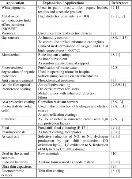
Application Explanation / Applications References

White pigments Used in paint, plastic, inks, paper, leather, textiles and cosmetic products

[7-11]

Metal oxide

semiconductor field effect transistor (MOSFET)

High dielectric constants (ε = 100) [9,11,12]

Varistors Used in ceramic and electric devices [8] Gas sensors As humidity control

[image:30.595.114.546.105.689.2]

To control the air/fuel mixture in car engines Utilized in determination of oxygen and CO at high temperatures (>600° C)

[8,9,11,13]

Biomaterials Bone implant coatings As bone substituent

As reinforcing mechanical support

[8,11]

Photo-assisted

degradation of organic molecules

Purification of waste water

Used in operating rooms in hospital Self-cleaning coating on car windshields

[7,8]

Anti cancer treatment Photochemical treatment [7] As thin film optical

interference coating

Antireflective coating Dielectric mirrors for lasers

Metal mirrors with enhanced reflection Filters

[7,8,9,11]

As a protective coating Corrosion resistant barriers [8,9,13] Photocatalysts (solar

cells)

Used in the production of hydrogen and electric energy

As anti-reflection coatings

[7,8,11,13]

Sunscreen As UV absorber in sunscreen cream with high sun protection factors

[7,9,11]

Food Foodstuff, food colouring (E-171) [9,11]

Pharmaceuticals As tablet coating, toothpastes [9,11] As catalysts Selective reduction of NOx to N2, Hydrogen

production by gas shift production, CO oxidation by O2, H2S oxidation to S, Reduction of SO2 to S by CO, NO2 storage

[9,11]

Used in fluxes and ceramics

Raw materials [10]

Li-based batteries Anatase form is used as anode material [8,11]

Ultra-thin capacitors [9]

Electrochromic devices

Thin film coating [8,13]

(31)

2-3

Fujishima et al. [7] explained about the critical role of TiO2. By using TiO2 in photocatalysis, the environment can be rendered clean and energy consumption can be

decreased. Table 2.2 lists the various applications of TiO2 as a photocatalysis [7].

Property/Function Category Applications

Self-cleaning

Materials for residential and office buildings

Exterior tiles, kitchen and bathroom components, interior furnishings, plastic surfaces, aluminium siding, building stone and curtains, paper window blinds

Indoor and outdoor lamps and related systems

Translucent paper for indoor lamp covers, coatings on fluorescent lamps and highway tunnel lamp cover glass

Materials for roads Tunnel wall, soundproofed wall, traffic signs and reflectors

Others Tent material, cloth for hospital garments and uniforms and spray coatings for cars

Air cleaning

Indoor air cleaners

Room air cleaner, photocatalyst-equipped air conditioners and interior air cleaner for factories

Outdoor air purifiers

Concrete for highways, roadways and footpaths, tunnel walls, soundproof walls and building walls

Water purification

Drinking water River water, ground water, lakes and water-storage tanks

Others Fish feeding tanks, drainage water and industrial wastewater

Anti tumour activity Cancer therapy Endoscopic instruments

Self-sterilising Hospital

Tiles to cover the floor and walls of operating rooms, silicone rubber for medical catheters and hospital garments and uniforms

Light + TiO2

[image:31.595.118.546.77.293.2]

titanium dioxide photocatalytic action fog-proof (frost-proof) anti-bacterial anti-viral, fungicidal water treatment water purification anti-soiling self-cleaning anti-cancer (photochemical cancer treatment) deodorising air purification

Figure 2.1: TiO2 photocatalysis general applications [7].

[image:31.595.115.548.417.782.2]

(32)

2.1.1.3 Biomedical Applications

TiO2 is used in biomedical applications as fine particles, coatings and oxide films on the

outer surface of biomaterials (Table 2.3). The surface of the Ti-based alloys forms

TiO2 layers in aqueous solutions in the human body and act as the interface for strong

bonding with natural connective tissue [14]. The TiO2 film also provides corrosion

resistance and contributes to improve biocompatibility of the implant [8].

Fujishima et al. [15] implanted cancer cells under the skin of mice to cause tumours to

form, and when the size of the tumours grew to about 0.5 cm, suspension containing

fine particles of titanium dioxide was injected into it. After 3 days, the skin was cut

open to expose the tumour and it was irradiated with ultraviolet (UV) and thus treatment

clearly inhibited the tumour growth. However, this technique was not effective in

stopping cancer which had grown beyond a certain size limit [15].

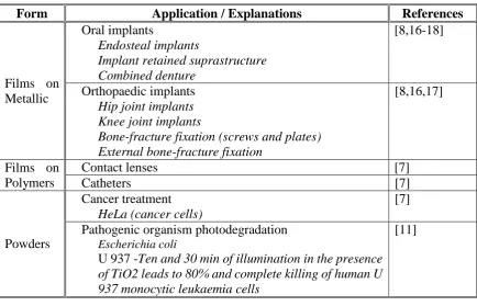
Form Application / Explanations References

Films on Metallic

Oral implants

Endosteal implants

Implant retained suprastructure Combined denture

[8,16-18]

Orthopaedic implants Hip joint implants Knee joint implants

Bone-fracture fixation (screws and plates) External bone-fracture fixation

[8,16,17]

Films on Polymers

Contact lenses [7]

Catheters [7]

Powders

Cancer treatment HeLa (cancer cells)

[7]

Pathogenic organism photodegradation

Escherichia coli

U 937 -Ten and 30 min of illumination in the presence of TiO2 leads to 80% and complete killing of human U 937 monocytic leukaemia cells

[11]

2.1.2 Crystal Structure and Phase Transformation

Titanium forms four well-defined oxides; monoxide (TiO), sesquioxide (Ti2O3), dioxide

or titanic acid (TiO2) called titania and pentoxide (Ti3O5) as shown in Figure 2.2.

[image:32.595.109.544.392.671.2]

(33)

2-5

(Tale 2.4). From a practical standpoint, the dioxide (TiO2) is the most important oxide

[19].

TiO2 exists in nature in the form of minerals like anatase, brookite and rutile. Rutile is

commonly found in nature; however, anatase and brookite are extremely rare.

Generally, TiO2 exist in an amorphous form at temperature below 350°C [9]. Above

that temperature, anatase phase is formed and at temperatures greater than about 800°C,

the most stable crystalline phase rutile, is formed [9,21].

According to Bokhimi [22], in most cases of TiO2 synthesis, anatase is the main phase

and brookite occurs as a minority phase, depending on synthesis conditions. The rutile

phase is obtained by annealing anatase and brookite at temperature higher than 500°C

[22]. The crystalstructures of the three oxide forms can be discussed further in terms

[image:33.595.174.510.140.409.2]

of orientation of the (TiO6₂ ) octahedral [11].

Figure 2.2: Phase diagram of the Ti-O system taken from Samsonov [20]. The region Ti2O3 - TiO2 contains Ti2O3, Ti3O5, seven discrete phases of the

(34)

Property TiO2 TiO Ti2O3

brookite anatase rutile

Colour dark brown white white bronze purple-violet

Melting point, °C - - 1830-50 1737 2127

Density (25°C), kg/m3

4170 3900 4270 4888 4486

Crystal structure orthorhombic tetragonal tetragonal Cubic rhombohedr al [24]

2.1.2.1 Anatase

Anatase which refers to the long vertical axis, was named by R.J. Hauy in 1801 from the Greek word „anatasis‟ meaning „extension‟ [11]. Anatase has a tetragonal

crystalline structure (Figure 2.3a) [22] and is built up from octahedra that are connected

at their edge (Figure 2.3b) [11].

[image:34.595.117.543.103.228.2]

(a)

Figure 2.3: Crystal structure of anatase [8,11,22].

102.308°

92.604°

Ti

[image:34.595.116.549.368.748.2]

O

Table 2.4: Properties of titanium oxides at various oxidation states [12,23].

(35)

2-7

2.1.2.2 Rutile

Rutile was discovered by Werner in Spain in 1803. Its name is derived from the Latin „rutilus‟ meaning red. Rutile is the most stable form of TiO2 [11]. Rutile has a crystal

structure with tetrahedral symmetry (Figure 2.4a) [22]. Rutile is built up from

octahedra that are connected predominantly at their edges (Figure 2.4b) [11].

[image:35.595.114.555.252.620.2]

(b)

(a)

Figure 2.4: Crystal structure of rutile [11,22].

90°

98.9°

3°

(36)

2.1.2.3 Brookite

Brookite was discovered by A. Levy in 1825 at Snowen (Pays de Gales, England) and it

was named in honour of the English mineralogist, H.J. Brooke [11]. Brookite has an

orthorhombic crystalline structure. The crystal structure can be described as distorted

octahedra with a titanium atom the centre and oxygen atoms in the vertices (Figure 2.5a)

[22]. Brookite is built up from the octahedra that are connected at their corner and

[image:36.595.111.555.277.614.2]

edges (Figure 2.5b) [11].

Figure 2.5: Crystal structure of brookite [11,22].

(a)

(b)

(37)

2-9

2.1.3 Thermodynamics and Phase Equilibrium

The thermodynamic phase stability in the Ti-O system is calculated based on

calorimetric data [11]. Based on minor differences in the Gibbs free energy (4-20

kJ/mole) value between the three phases, the most stable phase is believed to be rutile at

normal pressure and temperatures as compared to the other two phases. Particle size is

also known affect to the phase stability due to its association with surface energy and

surface stress. Thermodynamically, anatase is most stable at sizes less than 11 nm,

brookite between 11 and 35 nm, and rutile at sizes greater than 35 nm. The

transformation of anatase into rutile at room temperature is very slow and practically

does not occur. At macroscopic scale, the transformations of bulk TiO2 occur at temperatures more than 600°C.

The phase equilibria and crystal structures of the Ti-O system range between pure Ti

and TiO2 as shown in Figure 2.6. High solubility of oxygen in titanium (αTi) at low temperature leads to formation of Ti2O, Ti3O and possibly Ti6O. Ti2O has the anti-CdI2 structure with alternate oxygen layers vacant and additional vacancies randomly

[image:37.595.134.529.343.649.2]

(38)

structures are based on the NaCl structure. Four modifications of TiO have been

identified, αTiO, βTiO, αTi1-xO, and βTi1-xO [25]. The special points of the Ti-O

phase diagram are summarised in Table 2.5 and Table 2.6.

Phase Composition, at % O

Temperature

(°C) Reaction type

L + (αTi) ↔(βTi) 5 13 8 1720 ± 25 Peritectic

L ↔ (αTi) ~24 1885 ± 25 Congruent

Melting (αTi) + Ti3O2 ↔ Ti2O 33.3 40 33.9 ~600 Peritectoid (αTi) + Ti2O3 ↔Ti3O ~17 ~25 ~24.5 ~500 Peritectoid

L ↔ (αTi) + L ~37 ~31 ~53 ~1800 Monotectic (?)

L + (αTi) ↔ γ TiO ~55 31.4 34.5 1770 Peritectic

γTiO ↔ βTiO - ~1250 Unknown

βTiO ↔ βTi1-xO - Unknown

β Ti1-xO ↔ α Ti1-xO - Unknown

(αTi) + βTiO ↔ αTiO 33.3 51 50 940 Peritectoid

(αTi) + αTiO ↔ Ti3O2 32.4 50 40 920 Peritectoid

α Ti1-xO ↔αTiO + βTi2O3 54.5 50 60 460 Eutectoid

L ↔ γTiO + βTi2O3 ~57 54.5 59.8 1720 Eutectic

L ↔ βTi2O3 60 1842 Congruent

L + βTi2O3 ↔ βTi3O5 63 60.2 62.5 1770 Peritectic

βTi2O3 ↔ αTi2O3 60 ~180 Unknown

βTi3O5 ↔ αTi3O5 62.5 187 Unknown

γTi4O7 ↔ βTi4O7 63.64 -123 Unknown

β Ti4O7 ↔ α Ti4O7 63.64 -148 Unknown

L ↔βTi3O5 + ? ~64 62.5 - ~1670 Eutectic

βTi3O5 +βTi5O9 ↔ γTi4O7 62.5 64.29 63.64 ~1500 Peritectoid

L ↔ TiO2 66.7 1870 Congruent

L ↔ (βTi) 0 1670 Melting point

(βTi) ↔ (αTi) 0 882 Allotropic

transformation

There are five polymorphs of TiO2 that are anatase, brookite, TiO2–II, TiO2–III and rutile. Anatase and brookite are formed at low temperature and low pressure; TiO2–II and TiO2–III are formed from anatase or brookite under high pressure; and rutile is the stable phase at room temperature and pressure. The polymorphic transformations

anatase → rutile and brookite → rutile do not occur reversibly [30,31]. The magneli

phases are a series of discrete phases with stoichiometry TinO2n-1where n ≥ 2. The

magneli phases exist in between the monoxides (TiO) and dioxide (TiO2). Roy and

[image:38.595.107.545.184.598.2]