Solving Rank-deficient Linear Systems for the Estimation
of the Atmospheric Phase Delay Parameter
Vassilia Karathanassi
*, Arlinda Saqellari-Likoka
Laboratory of Remote Sensing, School of Rural and Surveying Engineering, National Technical University of Athens, 9 Heroon Polytechniou Street, 15780, Zographos, Greece;
*Corresponding Author: [email protected]
Copyright © 2014 Horizon Research Publishing All rights reserved.
Abstract
For each pixel, the values of the unwrapped phase produced by interferometric pairs can be parameterized and phase components, such as height, atmospheric path delay difference for the dates of every interferometric set image acquisition, and unwrapping error can be estimated through the solution of a rank deficient system of equations. There are several state of the art methods for solving rank deficient systems of equations, such as the Lower-Upper method, QR factorization and Singular Value Decomposition (SVD). In a previous work, the improved SVD method, which enables the accurate estimation of phase components, has been proposed. In this study, one alternative method for the estimation of the differential interferometry parameters, the improved QR, is proposed. The method relies on the reorganization of the system of equations by using external meteorological data which correspond to the acquisition dates that are less present in the interferometric SAR data set. All the aforementioned methods were tested and compared. The improved SVD and improved QR methods yield the most satisfactory results for all the phase components. The former estimates the heights by achieving almost GPS accuracy, whereas the latter is more robust, producing results of almost the same accuracy for all the estimated atmospheric path delays. However, the requirement of known values for at least two phase components makes the improved QR method less operational.Keywords
Interferometry, Atmospheric Path Delay, Dinsar, Rank Deficient Linear System1. Introduction
Water vapor is a key element of the hydrological cycle and the atmospheric greenhouse effect. The movement of water vapor through the hydrological cycle is strongly coupled to precipitation and soil moisture, which have important practical implications. SAR Differential Interferometry (DInSAR) observes microwave path delays due to
atmospheric effects and especially to those resulting from water vapor atmospheric contents. This enables the estimation of the total water vapor column with very high spatial resolution (e.g. 25m) on the ground. Although SAR satellites cannot provide sufficient temporal resolution, DInSAR can significantly contribute to the development of an integrated modeling for forecasting systems.
estimation of the surface deformation time evolution, and atmospheric signals are considered as artifact spurious terms. In this study the mathematical methods for solving rank-deficient linear systems that enable the estimation of the phase components involved in DInSAR models are evaluated. The study mainly focuses on the evaluation of the atmospheric phase delay component. Since this component when properly introduced in atmospheric models leads to water vapor calculation of the atmosphere, results of the research are very important for small-scale water vapor mapping of the atmosphere. These maps significantly contribute to the study of the microclimate of a region and climate of an entire area, as well as the monitoring of the climatic variability and changes.
Five mathematical methods for solving rank deficient systems: a) the LU decomposition method, b) the QR factorization method, c) the Improved QR factorization method, d) the Singular Vector Decomposition method, and e) the Improved SVD method [4], are applied and compared. All the methods are well documented in the literature apart from the Improved QR factorization method which is developed within this study. For each method, the appropriate algorithms in terms of applicability, reliability, accuracy, and efficiency have been developed. Comparison and validation of the results has been implemented through GPS and meteorological measurements.
2. Model for Interferometric Phase
Analysis
According to [4], the functional model which relates unwrapped interferometric phase
P
to the unknown parameters of height ΦΗ, atmospheric path delay due to changes in temperature, humidity and pressure for the dates of the interferometric set image acquisition, unwrapping errors Φerr, temporal decorrelation due to small changes either in the position or in the orientation of the individual scatterers (e.g. movement of the leaves in the trees) , deformation term ΦD [8, 9], and system noise , is given by (1):(1) The parameters and Φerrdepend on the coherence. Moreover Φerr and ΦΗ are a function of baseline and incidence angle. In the linear model (1), for every interferometric dataset the known parameter is the unwrapped interferometric phase. Considering that ground deformation does not exist in the area, and temporal decorrelation for coherent pixels, as well as system noise are very low, the parameters ΦD, and can be omitted [4]. Consequently based on (1), for n
interferograms and for a single pixel, the following system of
equations is considered:
(2)
In (2), the unwrapped interferometric phase is slightly affected by baseline inaccuracies in case that the SAR interferometric processing includes a rigorous orbital correction that corrects phase residual gradients in azimuth and distance on the interferogram and reflattening [10].
Using sensor parameters, such as the wavelength λ, the slant range r, the incidence angle α, and the perpendicular baseline , the unwrapped interferometric phase P can be converted into height [11]:
(3) Based on (2) equation (3) can be written as:
(4)
where and can be estimated for each pixel and interferogram. It is clear that errors in height due to the atmosphere and phase unwrapping depend on the baseline [12].
Based on (4), system of equations (2) can be written:
(5)
where, Hi is the inaccurate height provided by the unwrapped interferometric phase; B1.. Bn are the perpendicular components of the baselines of the interferometric sets; ΦΗi*Ci/Bi is the precise height Hpr without errors introduced by the baseline, incidence angle, atmospheric and unwrapping factors, and thus it has equal value for all the interferometric sets; and is the unwrapping error multiplied by the baseline and incident angle factors. For n interferograms and for the same ground pixel, can be considered the same in case that the same phase unwrapping algorithm is used, a baseline and an incident angle factor are introduced in the model and the coherence value of the pixel is almost the same for all the interferometric sets. Under the aforementioned conditions, system of equations (5) can be
Φ
attemp
Φ
Φ
sys= Φ + Φ + Φ + Φ + Φ
H at err D temp+ Φ
sysP
tempΦ
tempΦ
tempΦ
Φ
sys1 1 1
2 2 2
3 3 3
1
2
3
= Φ
+ Φ
+ Φ
= Φ
+ Φ
+ Φ
= Φ
+ Φ
+ Φ
= Φ
+ Φ
+ Φ
n n n
H at err
H at err
H at err
n H at err
P
P
P
P
iP
Β
⊥
(
sin
) / 4
H
=
P
λ
r
α
π
B
⊥⊥
= Φ + Φ + Φ( H at err) /
H C B
(
λ
sin ) / 4
α
π
=
C
r
1 1 1
2 2 2
3 3 3
1 1 1 1 1 1 1
2 2 2 2 2 2 2
3 3 3 3 3 3 3
* / * / * /
* / * / * /
* / * / * /
* / * / * /
= Φ + Φ + Φ
= Φ + Φ + Φ
= Φ + Φ + Φ
= Φ + Φ + Φ
n n n
H at err
H at err
H at err
n H n n at n n err n n
H C B C B C B H C B C B C B
H C B C B C B
H C B C B C B
* /
Φ
erriC B
i iΦ
iwritten as following:
(6)
In (6), is replaced by (the index i refers to the interferometric set), and by
. System of equations (6) can also be written as: H = K x (7) where H is the inaccurate height vector, K is the coefficient matrix, and x is the unknown parameter vector. The rank of the matrix K is equal to n because there are n interferograms which are independent, although they may result from interferometric pairs which may contain a common image. The unknown parameters
are k =n+2. Hence, the matrix K is an n × k, (k ≥n) matrix with k linearly independent columns, and has deficient rank.
3.
The Improved QR Factorization
Method
For system (7), each row of the matrix K is a vector that corresponds to an element of vector H. Elementary row operations do not affect the dependent relations between the column vectors. Moreover, in QR factorization, Q has the property that each ith (where i≤n) row of K can be expressed as a linear combination of m (where m≤k) columns of Q [13]. In the system of equations (7) combination can exist among any unknown parameter, such
as: .
However, because Hpr and Herr appear in all the equations of the system, they are the parameters that are estimated with the highest accuracy, and it is not suggested to be included in the linear combination. Thus, the optimum linear combination for the estimation of the unknown parameters should have the form:
(8) where , are elements of vector x. In case that Hat_ comb , is calculated by known atmospheric data then insertion of (8) in (7) reduces the rank deficiency of the matrix K by one, and yields more accurate solution. Besides, inclusion of a priori information related to atmospheric parameters significantly improves their estimation. The
parameter Hat_ comb can be calculated using (9).
(9)
where and are the absolute phase
delay for the dates that the master and slave image of the sets i and j are acquired. The values of absolute phase delay in (9) are obtained using known meteorological data, as well as the Saastamoinen model [14].
Equation (8) when inserted in (7) improves the accuracy of the solution. However, improvement is not similar for all the estimated atmospheric path delays. Accuracy is very high for the atmospheric path delays which appear in the sets i and j. This affects the accuracy of the other unknown atmospheric path delays since the total error of the QR factorization method is distributed among the unknown parameters [13].
In case that and (indexes i and j refer to interferometric sets) are not included in vector x, two more unknown elements, and are added in vector x, the rank deficiency of the matrix K increases by one, and equation (8) becomes:
(10) In fact, if the dates of the master and slave images of the sets n+1 and n+2 appear in the n interferograms, equation (10) is also a linear combination of the unknown atmospheric parameters and contributes to the improvement of the solution. But this time, high level of accuracy is not assigned to any unknown parameter of (7), and the total error is distributed among n+2 unknown parameters, instead of n. Both of the previous reasons contribute to the uniform distribution of the error. It is obvious that the increment of the rank deficiency of matrix K affects the total accuracy, which is expected to be slightly lesser than that produced by the inclusion of and in the combination.
In case that the selected dates for the master and slave images of the sets n+1 and n+2 appear the fewest times in the n interferograms, improvement of the accuracy is greater. The inserted linear combination leads to the following 1
2
..
, , ,.... ,
1 2
1
1
0
0
0
1
1
0
1
0
0
1
... ... ... ... ... ...
1
0
0
0
1
1
n
H H
H
pr
H Hat Hat Hatn Herr
=
⋅
* /Φat C Bi i
i Hati
* /
Φerr C Bi i i
Herr
, , ,.... ,
1 2
Hpr Hat Hat Hat Herr
n
, , ,.... ,
1 2
Hpr Hat Hat Hat Herr
n
comb i
at at atj
H
−=
H
−
H
i
at
H
H
at
j(
)
(
)
− − − − − − − − − − − − − − − − − − − − − − − − −= Φ
∗
−Φ
∗
− Φ
∗
−Φ
∗
i comb i i i i i j j j j j j at masterat at master at master
at master
at slave at master
at master
at master at master
at master
at slave at master
C
H
B
C
B
C
B
C
B
at-masterΦ
Φ
at-slavei
at
H
H
at jn+1
at
H
H
at n+21 2
−comb
=
n+−
n+at
at
at
H
H
H
i
at
system:
(11) In (11) the value of is estimated from meteorological data and it is known, whereas and
are considered unknown elements. The solution provided by (11) is improved in case that the SVD method is applied [15] on the QR factorization. In this case, the rank deficient matrix K is replaced by the (RTQT)-1 and the
inserted linear combination contributes to the generation of more accurate eigenvalues [13].
4.
Implementation, Results and
Evaluation
Interferometric process has been applied on eighteen ENVISAT images using the SARSCAPE tools. For these images, incidence angle varies from 18 degrees to 23 degrees. According to combination theory, 153 interferometric pairs can be formed from these images. However, only twenty five interferometric pairs were formed which have a perpendicular baseline component less than the 75% of the critical baseline and coherence value greater than 0.50. Their
baselines range from 46-751m. The mathematical approaches have been applied on a system of 25 equations provided by the unwrapped phase parameterization of the 25 interferometric pairs, respectively. This number was considered adequate for providing accurate solutions [4]. Four pixels, depicting the location of four meteorological stations respectively, were selected for the application of the mathematical methods. For these pixels, coherence value ranged from 0.53 to 0.71 and meteorological data were available for the dates that the ENVISAT images were acquired. Consequently, the methods were evaluated for 100 different atmospheric path delay values.
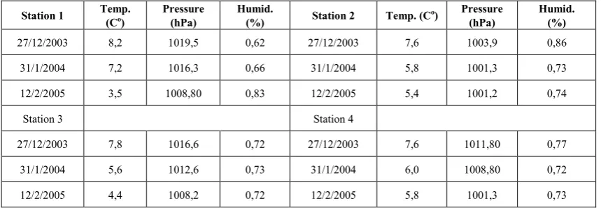
Five mathematical methods for solving rank deficient systems: a) the LU decomposition method, b) the QR factorization method, c) the Improved QR factorization method, d) the Singular Vector Decomposition method, and e) the Improved SVD method [4], were applied and compared. For the application of the improved QR method, meteorological data for three random dates were selected (Table 1), and for random couple combinations, atmospheric delays were estimated using the Saastamoinen model. The output of the linear combination of these atmospheric delays is calculated and inserted in the system of equations through a new equation.
[image:4.595.70.299.85.266.2]The solutions of the mathematical methods have been evaluated using a) height estimations based on GPS measurements, and b) estimated atmospheric path delays using known meteorological data as entries in the Saastamoinen model.
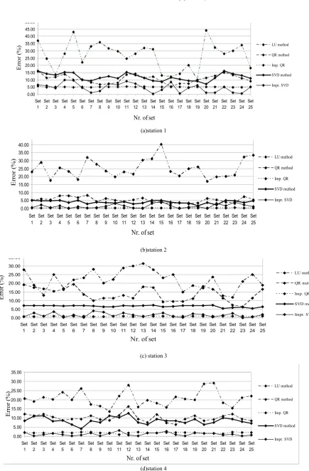
Figure 1 shows the percent atmospheric path delay errors produced by the five mathematical methods. In Table 2, the height error and the mean atmospheric path delay error (APDE), which was produced by each method, are shown for each meteorological station for each meteorological station. Moreover, Table 3 shows the minimum and maximum APDE for each station, produced by the Improved QR and Improved SVD methods.
Table 1. Atmospheric Data Used by the Improved QR Method.
Station 1 Temp. (Co) Pressure (hPa) Humid. (%) Station 2 Temp. (Co) Pressure (hPa) Humid. (%)
27/12/2003 8,2 1019,5 0,62 27/12/2003 7,6 1003,9 0,86
31/1/2004 7,2 1016,3 0,66 31/1/2004 5,8 1001,3 0,73
12/2/2005 3,5 1008,80 0,83 12/2/2005 5,4 1001,2 0,74
Station 3 Station 4
27/12/2003 7,8 1016,6 0,72 27/12/2003 7,6 1011,80 0,77
31/1/2004 5,6 1012,6 0,73 31/1/2004 6,0 1008,80 0,72
12/2/2005 4,4 1008,2 0,72 12/2/2005 5,8 1001,3 0,73
1
2
..
,
,
,
....
,
1
2
1
2
1 1 0 0 0 1 0 0
1 0 1 0 0 1 0 0
.. .. .. .. .. .. .. ..
1 0 0 0 1 1 0 0
0 0 0 0 0 0 1 1
,
,
comb n
at
H H
H H
pr
H H H
at at
H
at
H
err
H
at
H
at
n
n
n
−
=
+
+
−
⋅
-comb
at
H
1
+
n at
H
2
+
n at
[image:4.595.91.521.559.708.2](a)station 1
(b)station 2
(c) station 3
[image:5.595.88.524.44.707.2](d)station 4
Figure 1. Atmospheric path delay errors (%) produced by the five methods (a) station 1.(b) station 2. (c) station 3. (d) station 4. 0.00
5.00 10.00 15.00 20.00 25.00 30.00 35.00 40.00 45.00 50.00
Set
1 Set2 Set3 Set4 Set5 Set6 Set7 Set8 Set9 Set10 Set11 Set12 Set13 Set14 Set15 Set16 Set17 Set18 Set19 Set20 Set21 Set22 Set23 Set24 Set25 Nr. of set
E
rr
or
(%
) LU method
QR method
Imp. QR
SVD method
Impr. SVD
0.00 5.00 10.00 15.00 20.00 25.00 30.00 35.00 40.00
Set
1 Set2 Set3 Set4 Set5 Set6 Set7 Set8 Set9 Set10 Set11 Set12 Set13 Set14 Set15 Set16 Set17 Set18 Set19 Set20 Set21 Set22 Set23 Set24 Set25
Nr. of set
E
rr
or
(%
) LU method
QR method
Imp. QR SVD method
Impr. SVD
0.00 5.00 10.00 15.00 20.00 25.00 30.00 35.00
Set
1 Set2 Set3 Set4 Set5 Set6 Set7 Set8 Set9 Set10 Set11 Set12 Set13 Set14 Set15 Set16 Set17 Set18 Set19 Set20 Set21 Set22 Set23 Set24 Set25 Nr. of set
Er
ro
r (
%
) LU method
QR method
Imp. QR
SVD method
Impr. SVD
0.00 5.00 10.00 15.00 20.00 25.00 30.00 35.00
Set
1 Set2 Set3 Set4 Set5 Set6 Set7 Set8 Set9 Set10 Set11 Set12 Set13 Set14 Set15 Set16 Set17 Set18 Set19 Set20 Set21 Set22 Set23 Set24 Set25 Nr. of set
E
rr
or
(%
) LU method
QR method
Imp. QR
SVD method
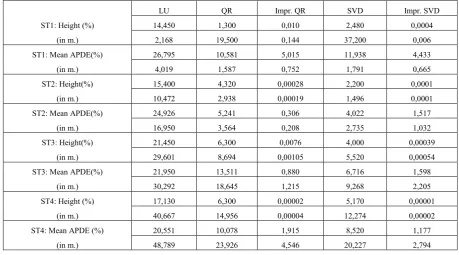
Table 2. Height and mean Atmospheric Path Delay Errors (APDE).
LU QR Impr. QR SVD Impr. SVD ST1: Height (%) 14,450 1,300 0,010 2,480 0,0004
(in m.) 2,168 19,500 0,144 37,200 0,006 ST1: Mean APDE(%) 26,795 10,581 5,015 11,938 4,433 (in m.) 4,019 1,587 0,752 1,791 0,665 ST2: Height(%) 15,400 4,320 0,00028 2,200 0,0001
(in m.) 10,472 2,938 0,00019 1,496 0,0001 ST2: Mean APDE(%) 24,926 5,241 0,306 4,022 1,517
(in m.) 16,950 3,564 0,208 2,735 1,032 ST3: Height(%) 21,450 6,300 0,0076 4,000 0,00039
(in m.) 29,601 8,694 0,00105 5,520 0,00054 ST3: Mean APDE(%) 21,950 13,511 0,880 6,716 1,598
(in m.) 30,292 18,645 1,215 9,268 2,205 ST4: Height (%) 17,130 6,300 0,00002 5,170 0,00001
(in m.) 40,667 14,956 0,00004 12,274 0,00002 ST4: Mean APDE (%) 20,551 10,078 1,915 8,520 1,177
(in m.) 48,789 23,926 4,546 20,227 2,794
Table 3. Minimum and Maximum APDEs Produced by the Improved QR and SVD Methods
Impr. QR Station 1 Station 2 Station 3 Station 4 Min. A.P.D.E.(%) 4,7 0,17 0,72 0,98 Min. A.P.D.E.(m) 0,71 0,12 0,99 2,30 Max. A.P.D.E.(%) 5,65 0,44 1,01 2,4 Max. A.P.D.E.(m) 0,85 0,30 1,39 5,63
Impr. SVD
Min. A.P.D.E.(%) 0,3 0,1 0,07 0,15 Min. A.P.D.E.(m) 0,70 0,07 0,10 0,02 Max. A.P.D.E.(%) 10,01 3,94 4,4 3,2 Max. A.P.D.E.(m) 23,49 2,68 6,07 0,48
Table 4. Classification of APD Errors for Each Method
(%) A.P.D. Error LU method QR method Impr. QR SVD method Impr. SVD [0 5 ](%) 0 10 98 18 90 [5 10 ](%) 1 45 2 60 10 [10 20 ](%) 25 32 0 22 0
[20 30](%) 45 3 0 0 0
> 30 (%) 29 0 0 0 0
Table 5. The Condition Number (CN) of the Matrices Used by Each Method
[image:6.595.76.537.350.744.2]It is observed that LU presents the lowest accuracy. QR factorization and SVD present higher accuracy, however up to 13% errors were produced, especially by the QR method and for estimations of the atmospheric path delays. Generally, height is more accurately estimated since it is the most encountered parameter in the rank deficient system of linear equations.
The improved QR and SVD methods yielded satisfactory results for both height and atmospheric path delays. The improved SVD method achieved almost GPS accuracy for height estimations. When using this method, the bounds of the eigenvalues of the pseudoinverse matrix are considered constant and new eigenvalues are added inside the bounds, but close to the bounds. The height parameter is defined by the higher eigenvalue which is one of the bounds, hence accuracy for height parameter is very high and improved SVD achieved the best performance regarding height estimation (Table 2). Moreover, it is observed that height accuracy is independent of the altitude of the point. However, the accuracy of the atmospheric path delay is not stable. For each station, atmospheric path delay estimations oscillate around a low mean value. For station 1 for example, whose solution is the most unstable in terms of accuracy, errors range from 0.3 to 10% (Table 3). Using the improved SVD method, 18 observations yielded an APD error 0-5%, 60 observations yielded an APD error that ranges from 5 to 10%, and for 22 observations the error ranges from 10 to 20% (Table 4).
The improved QR method yielded high accuracy and robust results regarding atmospheric path delay estimations (Fig. 1). For all the dates, the error was very low and almost similar. As it is observed in Table 4, the method yielded errors less than 5% for the 90 observations out of 100, i.e. the 98% of the observations. The combination of the two phase components that is inserted in the system through the new equation contribute in the production of two new eigenvalues within the eigenvalue vector and a) help the system to provide accurate solutions for the respective parameters, and b) define bounds of subintervals in the eigenvalue vector, producing this way more accurate estimations for all the atmospheric path delay parameters.
The methods were also evaluated by the condition number of the matrices used for the solution of the problem. Condition number is an important index that shows the accuracy of the solution provided by each method. The calculation of this index is based on [16]. It is observed that LU, QR and SVD produce ill-conditioned matrices (Table 5). So, the solutions that they provide have considerable errors. In contrast, Improved QR and Improved SVD produce well conditioned matrices which may lead to more accurate solutions. Condition numbers with values greater than 0.61 can be considered adequate in case that rank deficient matrices are evaluated. Improved SVD is the method that presents the closer to 1 condition number values thus confirming the stability of the solution.
5. Conclusions
In this study the unwrapped phase produced by interferometric pairs has been modeled for estimating height and atmospheric phase delay difference for the dates of every interferometric set image acquisition. Although the assumption that phase unwrapping errors under specific conditions can be considered the same for all the observations has been made, which is not fully true, the results in terms of height and atmospheric delay accuracies are promising. For solving the unwrapping phase model, different mathematical methods have been evaluated. Three basic linear algebraic methods that solve rank deficient systems have been considered: the Lower-Upper (LU) factorization, the QR factorization and the Singular Value Decomposition (SVD) method. Among these methods, the SVD method yielded the best performance, although it did not achieve the highest accuracies. The study has shown that performances do not depend on the characteristics of the considered targets (pixels) but mainly on the mathematical method used.
Furthermore, an improved QR method for solving rank deficient system was proposed, which exploits linear combinations among the atmospheric parameters of the unwrapped interferometric phase model. Thus, meteorological data for at least three dates, ideally the most rarely encountered among the dates of the SAR image acquisitions, are required. The high accuracy of the inserted meteorological data forces the method to produce high accuracy.
The method has been compared with the improved SVD method. The accuracy provided by both methods is quite satisfactory for height and atmospheric path delay estimations. However, their use is addressed to different applications. For the production of an accurate DEM, the improved SVD method is the recommended method because it yields very accurate heights. Atmospheric path delay values, which lead to the water vapor estimation, are satisfactory estimated by the improved SVD method, but their error is not uniform ranging from 0.3% to 10% in the experiments undertaken in this study. On the other hand, the improved QR method yields quite accurate path delay values with a uniform distribution of the error. Its use fits well the requirements of meteorology and climatic change studies. However, the need of prior knowledge of meteorological data for at least three dates may be considered as a significant constraint in its operational application.
Acknowledgments
ENVISAT SAR acquisitions were provided by ESA-11703.
REFERENCES
S.Waugh, T. Veneboer, G. Puglisi, M. Mattia, D. Baker, S.C. Edwards, S.J. Edwards, P.J. Clarke, “Atmospheric models, GPS and InSAR measurements of the tropospheric water vapour field over Mount Etna,” Geophysical Research Letters, vol. 29, no. 19, pp. 1-11, 2002.
[2] Xiao-li Ding, Zhi-wei Li, Jian-jun Zhu, Guang-cai Feng, and Jiang-ping Long, “Atmospheric Effects on InSAR Measurements and Their Mitigation,” Sensors, Vol. 8, pp. 5426-5448, 2008.
[3] S. Knospe, “Covariance Estimation for dInSAR Surface Deformation Measurements in the Presence of Anisotropic Atmospheric Noise,” IEEE Transactions on Geoscience and Remote Sensing, vol. 48, no. 4, pp.2057-2065, 2010. [4] A. Saqellari-Likoka, V. Karathanassi, ”An approach for
solving rank-deficient systems that enable atmospheric path delay and water vapour content estimation,” IEEE Transactions on Geoscience and Remote Sensing, vol. 46, no. 10, pp.3187-3195, 2008.
[5] P. Berardino, G. Fornaro, R. Lanari, E. Sansosti, “A new Algorithm for Surface Deformation Monitoring Based on Small Baseline Differential SAR Interferograms,” IEEE Transactions on Geoscience and Remote Sensing, vol. 40, no. 1, pp. 2375-2383, 2002.
[6] O. Mora, J.J. Mallorqui, A. Broquetas, “Linear and nonlinear terrain deformation maps from a reduced set of interferometric SAR images,” IEEE Transactions on Geoscience and Remote Sensing, vol. 41, no. 10, pp. 2243-2253, 2003.
[7] S. Usai, “A Least-Square Approach for Long-term Monitoring of Deformations with Differential SAR Iterferometry,” in Proc. International Geoscience and Remote Sensing Symposium 2002, Toronto, Canada, June 24-28, 2002, vol. 2, pp. 1247-1250.
[8] D. Just, and R. Bamler, “Phase statistics of interferograms
with applications to synthetic aperture radar”, Applied Optics, vol. 33, no. 20, pp. 4361-4368, 1994.
[9] R.F. Hanssen, H. Zebker, R. Klees, S. Barlag, “On the use of meteorological observations in SAR interferometry,” In Proc. International Geoscience and Remote Sensing Symposium 1998, Seattle, Washington, USA, July 6-10, 1998, pp.1644-1646.
[10] A. Lugli, “Orbital refinement”, in Interferometria SAR per lo studio di movimenti e generazione di modelli digitali del terreno in Antartide, Università di Bologna, 2010, ch 18,pp. 128-132.
[11] G. Fraceschetti, and R. Lanari, “Coding Issues,” in Synthetic Aperture Radar Processing, CRC Press, Taylor and Francis group, Boca Raton, 1999, ch. 1, pp. 31-33.
[12] K. S. Rao, H. K. Al-Jassar, S. Phalke, Y. S. Rao, J.-P. Muller, and Z. Li, “A study on the applicability of repeat-pass SAR interferometry for generating DEMs over several Indian test sites,” International Journal of Remote Sensing, vol. 27, no. 3, pp. 595 – 616, 2006.
[13] G. Strang, “ Linear Algebra and its Applications”, 4th Edition, Publisher: Brooks Cole, 2005, pp 544.
[14] J. Saastamoinen, “Contribution to the Theory of Atmospheric Refraction,” Bulletin Geodesique, pp. 105-107, 1973. [15] J. Chen, K. Ji, Z. Shi, W. Liu, “Implementation of Block
Algorithm for LU Factorization,” In Proc. 2009 World Research Institutes (WRI) World Congress on Computer Science and Information Engineering, Los Angeles, California, USA, 31 March - 2 April 2009, vol. 2, pp. 569-573.