110
Journal of the Statistical and Social Inquiry Society of Ireland Vol. XXXIX
Structural Economic Change in Ireland 1957-2006: Statistics, Context and Analysis
Patrick Quill1 The Central Statistics Office
Paddy Teahon
formerly Secretary General, Department of the Taoiseach
(read before the Society, 21 January 2010)
Abstract: The fifty years since the publication of Economic Development has been a time of change and growth for Ireland. Analysis of the development of the structural composition of the economy in this period requires a consistent and comprehensive dataset from the late 1950s onwards. The national income and expenditure tables have changed over time and a consistent set of historical tables is only available from 1970 onwards. Gross value added by sector in the official historical series is given for only a small number of sectors. In this paper the tables of gross value added by sector in current and in constant prices, are extended backwards to 1957 and expanded to include fifteen industry groupings. A new comprehensive and consistent dataset spanning fifty years of the Irish economy is thus constructed. Details of the methods and sources used to develop these series are presented. A context for analysis is set out based on the framework or model developed by Professor Carlota Perez in a series of publications since 1983 and most notably in her 2002 book Technological Revolutions and
Financial Capital. Structural changes of the economy over the period are analysed. The analysis shows
how different sectors have contributed to the economy over time. It also reveals, in the Irish case, that structural change can be independent of economic growth. The Irish economy is set in the context of the Perez model of technological revolutions and Ireland‟s place in current and past technological revolutions is evaluated.
Keywords: economic development, structural change, historical data
JEL Classifications: E01, L16, O11
1.INTRODUCTION
This paper develops a set of statistics so as to identify the structural composition of the Irish economy from 1957 to 2006. The decline of some sectors and growth of others over the 50 year span in Ireland is examined within the framework or model of technological revolutions set out by Professor Carlota Perez in a series of publications over the years since 1983 and most notably in her book Technological Revolutions and Financial Capital [14].
To analyse structural economic change requires detailed statistics over a long time period and a context within which to analyse that change. Developing the statistics for gross value added in current and constant prices for the fifty years since 1957, outlining a context based on the Perez model and analysing the statistics in that context are the subjects of this paper.
111
The paper is in seven sections
o This introduction
o The 5-sector extended historical series 1957-2006
o Constructing a 15-sector series
o The context which outlines the Perez approach and how it is relevant to the Irish case
o The main results and analysis
o The Irish Experience in the context of the Perez model
o Conclusions, some policy implications and future work.
The value of the work presented in the paper is twofold: the series developed stand on their own as an important extension of those currently available both in terms of the length of the series and of the sectoral coverage now available; the analysis is a first step in understanding how technology impacts not just on individual sectors such as computers, chemicals or software but on the entire economy and provides thinking on how policy should be advanced so that Ireland might benefit from opportunities which will arise in the years ahead. Additionally the paper provides the basis for further work described in Section 7.
The series produced is an extension of the national accounts series of gross value added by sector. A long series makes different types of analysis possible. Time series decompositions are best performed using a long dataset - over 20 data points are recommended. Due to inconsistencies over time of the official national accounts series, analysis that depends on longitudinal data is not always possible. The UK suffers from the same breaks in some of their time series as we do, due to changes in national accounting introduced in 1997 and Martin [10] recently produced methods for constructing a historical series of the institutional sector accounts for the UK.
This is also the most detailed series of GDP by sectoral composition available. The significance of structural factors in understanding the Irish economy is demonstrated by Keating [6], who warns against examining productivity and economic growth without regard to the effect of the increasing importance of some sectors and the corresponding decline in the importance of others.
The data assembled thus stand alone as a new and useful dataset. It is of obvious interest to macroeconomists, but it is also likely to be of use in, for example, environmental economics for relating sectoral emissions to output. The authors hope that it may be used as such. The complete set of tables is available on request from the authors and is presented in Excel format on the Statistical and Social Inquiry Society of Ireland (SSISI) website. It provides a sound basis for discussion of the structural changes in the Irish economy over the last 50 years. The figures are derived mainly from data which are publicly available either in hard copy as in the case of the older series or in electronic form on the CSO website. The data however are not a replacement for official published statistics.
Using the Perez technological approach in the analysis is a first step in understanding how technology has impacted on Irish structural change.2 There are two broad existing perspectives on how structural change, especially recent rapid change, has been influenced in the Irish case. Many economists including Patrick Honohan and Brendan Walsh [5] and Cormac Ó Gráda [13] view the recent boom as delayed convergence that made up for lost ground caused by macroeconomic, especially public financial, mismanagement. Frank Barry [10] in a perspective closer to the present paper and referencing Krugman argues that the increased foreign direct investment inflows represented the one essential condition accounting for the strength of the boom. Clearly public policy and foreign direct investment are both important. Technology is recognised to be important at a general level. Arguably, however, understanding the impact of technology from a global perspective and how that impact diffuses from leading countries to a follower country such as Ireland can be equally important, especially in providing thinking on how supply side policy should have been and should be advanced to gain from the challenges and opportunities Ireland has faced and will encounter in the years ahead and in understanding how structural change takes place in different phases of foreign direct investment and in different domestic macroeconomic conditions.3
2
Professor Perez, who has read a draft of this paper, writes in private correspondence with the authors that it is „courageous attempt at using statistics to explain and illustrate the Irish experience.‟
3
112
Review of some related literature and commentaryStructural change in the Irish economy has been considered in some recent articles. Sexton [19] considers changes over the period 1995 to 2005. His article looks at the broad economic sectors presented in tables 3 and 4 of the current National Income and Expenditure (NIE) publication with the industry sector broadened out to include the modern sectors of software reproduction, chemicals and electronics. Sexton presents constant price tables of gross value added for 7 sectors in the economy. A large part of his discussion is a comparison of productivity across the sectors over time. Our paper expands the work done by Sexton. We concentrate also on the presentation of the economy in table 3 and 4 of the NIE. Our tables increase the sectors considered to fifteen and the series extends backwards to 1957. Our main interest is in the changes in the shares of sectors and their contributions to economic growth. Although productivity is readily derived from the constant price tables by using estimates of employment, we do not deal with it in this article.
McCarthy and O‟Leary [11] look at structural drivers of economic growth. Their work considers a series, in current prices, over the period 1995-2000. Eight sectors and their contribution to GNP are considered. Industry is treated as one sector. One decision that McCarthy and O‟Leary make is to omit the value added from rent and imputed rent from the calculations. This may have been worthwhile in their consideration of productivity. In the current paper we include rent as a component of GDP. In doing so, our tables are fully compatible with the national accounts. In fact we have chosen to amalgamate construction with real estate, rent and imputed rent, to be able to identify as a whole the contribution of property related activities to growth in the Irish economy. Another aspect of the McCarthy and O‟Leary article is that, after apportioning net factor income, estimates of GNP by component sector are derived. Our paper concentrates only on the components of GDP, by sector.
2. THE 5-SECTOR HISTORICAL SERIES 1957-2006
Background
In 2005 the national accounts division of the Central Statistics Office produced a revised historical series for the National Income and Expenditure (NIE). This historical series is available on the CSO website and contains a complete and consistent set of NIE tables showing all national accounts aggregates from 1970 to the present. The only exception to the consistency of the tables is that aggregates before 1995 are shown without financial intermediary services indirectly measured (FISIM) whereas those since 1995 are with FISIM causing a break in the series. (The concept of FISIM is explained briefly in the next section.)
Tables 3 and 4 of this series present GDP broken down by broad economic sector in current and chain-linked constant prices. The contribution to GDP by a given sector is called its gross value added (GVA). GDP is comprised of the sum of all sectors‟ GVA plus taxes less subsidies. The national accounts historical series identifies five sectors‟ GVA (more recent years of the national accounts constant price series broaden to ten sectors). In this section we extend the tables of GVA by sector backwards to 1957.
Our sources are: Appendix 4 of NIE1977 which contains tables for 1960 to 1970; NIE1965 containing tables of GDP for the years 1958 to 1960; and NIE1961 with tables for the expenditure, but not the income, components for 1957. The main issue here is that accounting practices have changed over time. Two significant changes to the accounting principles used in national accounts were the introduction of the European System of Accounts of 1995 (ESA95) in 1998 and the introduction of FISIM in 2003. The historical tables on the CSO website are compiled according to ESA95 rules but do not include FISIM for years before 1995. To extend the whole series back to 1957, we make estimates of the effect of these accounting principles on published data based on both accounting practices. We compare, for example, published versions of GVA with FISIM with published versions of GVA without FISIM. These findings are used to correct the full series without FISIM to account for the changes that the introduction of FISIM imposes upon them. In the more detailed tables we scale the sub-sectors‟ GVA up to the corrected broad sectors GVA.
113
A second issue for years before 1970 is converting base year constant prices to a constant price series in previous years‟ prices. This is done by assuming for each broad sector that the two types of constant price series are equivalent.
Methodology - current prices
The classifications at broad sectoral level comprise five sectors: Agriculture forestry and fishing; industry including building; distribution, transport and communication; public administration; and other services. This classification system has been in place since 1958. We link the older table to the historical series at current prices by making estimates of the effect of the transition to ESA95 accounting and the introduction of FISIM.
To convert to ESA95 proceed as follows: The components of the current price series are adjusted individually according to the following factors found in the historical series (at ESA95) and the NIE 1977 (which is compiled pre ESA95):
NIE1977
1974)
-(1970
value
component
average
weighted
NIE
hist
1974)
-(1970
value
component
average
weighted
(where the weights 16:8:4:2:1 are applied to the years 1970 to 1974 respectively).
FISIM (financial intermediary services indirectly measured) was first used in the national accounts in NIE2005. FISIM measures the value gained by banks and lending institutions through lending and borrowing with ordinary customers at a different rate of interest than with financial institutions. Before the introduction of FISIM into national accounting the banking sector‟s GVA from this activity was not recognised. For this reason CSO attributed a value added to these institutions in the sectoral breakdown in NIE table 3. This attributed value added is the „adjustment for financial services‟ that was then deducted from the calculation of GDP. It follows that we are on firm footing if we use the adjustment for financial services as an indication of FISIM.
Financial institutions, within the other services sector, are receivers of FISIM. All other sectors as well as households pay FISIM (FISIM is also imported and exported). We consider the NIE tables for 1995 to 2005 with FISIM and the same tables without FISIM. For each sector we calculate the average, over 1995 to 1999, of the ratio of the effect of FISIM from the former table with the adjustment for financial services in the latter. Since all preceding years after 1959 have an adjustment for financial services, we use this ratio to adjust the five sectors for the effect of FISIM. The effect is as follows: The GVA of the other services sector‟s (which includes banks) is increased as it is a net recipient of FISIM, whereas all other sectors‟ GVA is reduced as FISIM is added to each industry‟s costs. The total GVA is increased. This is because some of the FISIM is paid by households and government.
It appears that the tables for 1957-1959 are presented with FISIM (see note (i) on page 4 of NIE 1976). So there is no work to do in this case.
114
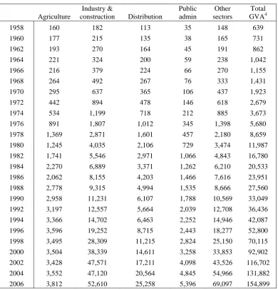
Table 2.1 Extended Historical Series, Current Prices: GVA by sector of origin at current market prices 1958 -2006 (€m)
Agriculture
Industry &
construction Distribution
Public admin
Other sectors
Total GVA4
1958 160 182 113 35 148 639
1960 177 215 135 38 165 731
1962 193 270 164 45 191 862
1964 221 324 200 59 238 1,042
1966 216 379 224 66 270 1,155
1968 264 492 267 76 333 1,431
1970 295 637 365 106 437 1,923
1972 442 894 478 146 618 2,679
1974 534 1,199 718 212 885 3,673
1976 891 1,807 1,012 345 1,398 5,680
1978 1,369 2,871 1,601 457 2,180 8,659
1980 1,245 4,035 2,106 729 3,474 11,987
1982 1,741 5,546 2,971 1,066 4,843 16,780
1984 2,270 6,889 3,371 1,262 6,210 20,533
1986 2,062 8,155 4,203 1,466 7,616 23,951
1988 2,778 9,315 4,994 1,535 8,666 27,560
1990 2,958 11,231 6,107 1,788 10,569 33,049
1992 3,197 12,557 5,664 2,039 12,708 36,436
1994 3,366 14,702 6,463 2,252 14,946 42,087
1996 3,596 19,252 8,715 2,443 18,277 52,800
1998 3,495 28,309 11,215 2,824 25,150 70,115
2000 3,504 38,339 14,611 3,258 33,853 92,902
2002 3,428 47,571 17,211 4,098 43,526 116,702
2004 3,552 47,120 20,564 4,845 54,966 131,882
2006 3,812 52,610 25,258 5,396 69,097 154,899
Methodology – constant prices
Traditionally national accounts constant price series were constructed as Laspeyre‟s volume indices with base weights updated every 5 years, or more. This was the practice in most statistical offices. In recent times, especially since the impact of hi-tech industry and globalisation, it is found unsatisfactory to use prices fixed for long periods and statistics offices have switched to using chain-linked constant price series with goods valued at previous years‟ prices (see Sexton [18] for a discussion of this point). To convert the base year constant price series, as published, to ESA95 accounting, we adjust each constant price component by the ratio of the current price component in ESA95 to the same component in current prices pre ESA95.
To convert from tables in base year prices to tables in chain linked previous year prices, we make the following assumption: For each sector, the ratio of the GVA of this year to that of last year, measured in last year’s prices, is equal to the ratio of the GVA of this year to that of last year measured in the
base year’s prices. This assumption, which implies no difference between the prevailing convention of
constructing constant price series (in previous year prices) and that used before 2003 (using a base year) is necessary to maintain the growth rates presented in the official national accounts. As we are dealing with historical, pre-electronic age data, there are grounds for accepting the assumption, as changes in prices are likely to have been relatively homogeneous at this time across the different sectors.
4
115
Converting the constant price series for 1960-1995 to a series with FISIM is done in the same way as the current price series.
[image:6.595.112.486.194.600.2]This concludes the work done to extend the constant price historical series. Growth rates in the extended historical series are close to growth rates in the official statistics (after 1995 the growth rates are equal to the growth rates in table 4 of NIE 07). Any differences are due to the effects of transition to ESA95 accounting with FISIM. Every second year of the series is presented in Table 2.2.
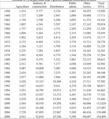
Table 2.2 Extended Historical Series, Constant Prices: Sectoral GVA at previous year's prices, chained, referenced to 2006
Agriculture
Industry &
construction Distribution
Public admin
Other sectors
Total GVA
1958 1,514 2,777 2,724 1,967 10,255 15,950
1960 1,727 3,200 2,967 2,009 10,908 17,711
1962 1,758 3,700 3,286 2,092 11,372 19,162
1964 1,807 4,244 3,587 2,167 12,142 20,818
1966 1,737 4,521 3,751 2,205 12,294 21,329
1968 1,890 5,364 4,272 2,315 13,089 23,939
1970 1,902 5,825 4,814 2,495 13,976 25,717
1972 2,172 6,469 5,251 2,770 15,713 28,778
1974 2,264 7,121 5,799 3,118 16,898 31,229
1976 2,235 7,284 5,847 3,324 18,263 32,583
1978 2,491 8,569 6,770 3,546 20,338 37,204
1980 2,349 9,370 7,322 3,881 22,123 40,812
1982 2,512 9,781 7,177 4,058 23,049 42,902
1984 2,887 10,608 7,083 4,066 24,515 45,016
1986 2,616 11,252 7,215 4,201 25,263 46,448
1988 2,927 13,006 7,846 4,046 26,102 49,509
1990 3,428 15,315 10,560 4,210 27,511 57,582
1992 3,627 16,633 9,621 4,278 29,756 60,017
1994 3,253 18,795 10,512 4,235 31,636 64,862
1996 3,570 23,927 13,372 4,367 34,370 77,781
1998 3,670 31,658 15,993 4,490 39,617 93,489
2000 3,564 38,970 19,558 4,681 46,066 112,020
2002 3,523 45,268 21,972 5,019 52,455 127,857
2004 3,728 47,895 22,967 5,249 60,436 139,480
2006 3,812 52,610 25,258 5,396 69,097 154,899
3. CONSTRUCTING A 15-SECTOR SERIES
116
ClassificationsThe 15 industry groupings are chosen to best represent, in summary form, the sectors of significance to the Irish economy and the sectors of significant change in the period. They are as follows:
Code NACE Description
1 01, 02, 05 Agriculture, forestry, fishing
2 15 Food products
3 24 Chemicals
4 30 - 33 Electronics
5 10-21,23,25-29, 34-41 Other industry
6 40 Energy
7 45, 70 Building, real estate, rent and imputed rent
8 50-52 Distribution
9 55 Hotel & restaurant
10 60-63 Transport
11 64 Communications
12 65-67 Financial
13 22 & 72 Printing, software and computers (IT)
14 71-74, 91-95 Other services
15 75 - 90 Public services
We disaggregate distribution, transport and communications. Hotel and restaurant services are isolated specifically as a barometer of the tourism industry. As mentioned above, in order to better examine the effect of property on the economy, we amalgamate construction with real estate and rent of dwellings (real and imputed). We use the name „electronics‟ to cover the manufacture of office machinery, computers, processing chips and communication, medical and precision instruments, this is NACE 30-33. NACE 22 (printing, reproduction of recorded media including software) is amalgamated with NACE 72 (computer services). Here we combine a manufacturing activity with a service. This is in line with the forthcoming NACE Rev 2 where all computer related activities are classified together. Education, health and public administration are combined being for the most part non-market government sponsored activities.
Methods used to compile a current price series
Most statistics compiled by the CSO are in current prices so constructing a current price series is, in theory, a straightforward task. A long series has, however, two particular difficulties: the classifications and groupings of industries used to compile the statistics do not stay fixed over time; and the level of detail is uneven across different sectors. For the purposes of comparing data from different years, these issues – classification and varying levels of detail - are addressed.
The NACE coding is an international classification of industries which was adopted by the CSO in compiling 1973 statistics. The original NACE coding was replaced by NACE Rev1 in 1995. Before NACE, it appears each country had its own individual classification of industries. Thus there are three different classifications used by CSO in the period from 1957 to the present. In Part 1 of the paper we construct the tables according to prevailing NACE Rev 1 classification (with amalgamations). For earlier classifications we compile data at the highest level of detail possible. The accounts are then reassembled to NACE Rev 1 groupings.
117
ESA95 with FISIM tables exactly compatible with later tables. In the input-output tables data are available at a good level of detail. The Statistical Abstract has data on tourism, education, health, and public administration (also for construction up to 1973). The CSO website makes available in electronic form most CSO published statistics in Database Direct. Publications from various external sources such as the Department of Environment and Bord Fáilte are also used. Although many of these sources do not present GVA for the whole sector we have been able to adapt them to our needs to produce the tables.
Methods used to compile a constant price series
We extend the historical national accounts series of GVA at chain linked constant market prices (table 4 of NIE) backwards to 1957. We further expand the series so as to include the GVA of a wider range of industries. Chain linking requires compiling accounts at a high level of detail in current prices and in prices of the previous year. We outline the method in the following paragraphs.
Using indicators of year-on-year volume growth or otherwise, each sub-industry‟s GVA is expressed in previous years‟ prices. These accounts are aggregated to industry, industry-group or sector level giving again the value of GVA for the aggregation in previous years‟ prices. Indices of the ratio of each year‟s GVA in previous years prices to the GVA of the previous year (in current prices) are found. These indices are linked by multiplication. Once this series of indices is made, a reference year is chosen. All years‟ GVA are expressed in terms of the prices of the reference year. The process is presented symbolically as follows:
Let
s
1,
s
2,
s
3,...
be an industry‟s sub-components with gross value added for year t given as,...
,
,
2 31
t t t
gva
gva
gva
where0
t
n
(where there are n + 1 years in our series).For each sub-component
s
i, letr i
pyp
gva
_
be the GVA in year r expressed in previous year‟s prices.We find the ratio of the sum of the GVA‟s in previous years‟ prices on the sum of the previous years‟ GVA‟s:
i r i i
r i r
gva
pyp
gva
I
1_
(1)
where the sum is over the sub-components. The indices are next linked by multiplication.
Given indices
I
1,
I
2,
I
3,...
thenI
1,
I
1I
2,
I
1I
2I
3,...
is the chain-linked series. The process is done for each component and for GDP itself. For this reason the components do not generally add exactly to GDP.In summary, to construct a constant price series in previous year prices, we need a set of accounts in current prices as well as a method of compiling these accounts in previous years‟ prices. Two methods are used: volume indices can be used to project forward the GVA of last year or price indices can be used to deflate this year‟s GVA to last years‟ prices.
In our work, we generally project forward GVA using volumes of production. The formula above is used to construct indices for each industry. The industries are then summed to each broad economic sector and scaled to the constant price series so that the year on year growth of the whole sector matches that of the five-sector historical series. That is, we start the work from first principles using detailed accounts of output, GVA and volume. Indices are constructed but adjusted so that, at the broad economic sector level, the growth rate presented in the official national accounts is maintained.
118
Where higher level detail is unavailable then a constant price series valued at a given base year‟s prices are used for the whole industry group. This is valid if the industry‟s components‟ prices are relatively stable over the period of the index. It is also valid if the price structure of the industry is relatively homogeneous i.e. that there is a good positive correlation between the individual products‟ prices. Furthermore in the case of a short index of volume, the ratio of successive years‟ constant prices is likely to be close to the year-on-year volume growth. In this case, however, the series produced is equivalent to the original constant price series.
Details by sector of methods used with reference to sources
In this section we present an inventory of the sources and methods used to produce the 15 sector disaggregation of the tables of GVA in current and constant prices for the years 1957 to 2006. The main sources are: the CSO‟s Statistical Abstracts for early years and Database Direct for later years, Censuses of Distribution and Censuses of Population as well as input-output tables. Briefly our method is as follows. For the current price tables we assemble GVA at the highest level of detail possible and re-aggregate to sector level. For the constant price tables we again assemble data at the highest level of detail and use volume indicators to express accounts in previous years‟ prices. Formula (1) is then used to construct the chain-linked series.
NACE 1-5 Agriculture
Value added of the agriculture, forestry and fishing sector at current and constant prices are already provided in the extended historical series.
NACE 10-14 Manufacturing and energy 1957-1972
The CSO„s Statistical Abstract for the years 1960 to 1974 contains the table „Industrial Production: Output, Cost of Materials, Salaries and Wages and Persons Engaged in each Industry‟. This table presents gross output, cost of materials and net output for 47 industrial sectors as well as for construction, energy production and local government. Net output is the difference between the gross output and the cost of materials used (including fuel). Net output for an industry type is greater than value added by the cost of services purchased by that industry.
Input-output tables give details of all inputs into each industry type. The service inputs omitted from the industrial production tables can be estimated using the input-output tables. Published input-output tables are available for 1964, 1969 and 1975. Tables for 1956 and 1960, constructed by Eamon Henry [4], are also available. For these benchmark years, the ratio of service inputs to material inputs is available. In the case of other years we estimate the ratio of service to goods inputs using the benchmark ratios and straight line methods.
By combining these ratios with data in the industrial production table, service inputs and GVA by industry type can be derived. We note that the inputs given in the input-output tables are domestic inputs with imports shown separately. We can assume however that there are no service imports of any significance in this time period so that the method employed here to estimate services is acceptable. We aggregate GVA by detailed industry type to NACE groupings and scale to the manufacturing and construction sector of the historical current price table already constructed. This gives a table of current price GVA by NACE groupings consistent with the historical series. Construction is scaled to the input-output value for construction (see below) and industry is scaled to the remainder of the „industry‟ category in the historical current price tables.
A further table in the same section of the Statistical Abstract provides the same industries‟ volume of output at 1953 prices. This is a rather long series at constant prices (running to 1973), but is adequate to calculate the year-on-year change at a detail needed to construct the chain-linked series. The chain linked series is constructed using the method outlined in section 2. (This is the method used throughout this section: For each NACE grouping we have GVA in current prices and the GVA in previous years‟ prices. Indices are found for each industry grouping using Formula 1. Finally, the indices are scaled to the 5-sector indices derived from the extended historical series.)
1973-1990
For 1973 to 1990, tables from the Census of Industrial Production are available on the CSO‟s Database
Direct. These tables use the original NACE classification. We distinguish between net output and GVA
119
indication of GVA but is not as complete in the coverage as the local unit file. Tables of volume of output are also available. For each industry type at a detailed sectoral level we compile GVA and GVA in previous years‟ prices. Each of the detailed sectors maps into a 2-digit NACE Rev1 code.
As a control total, we check that the GVA of manufacturing industry plus construction equals the GVA of „Industry‟ in the historical series. When construction as calculated below is subtracted from the total for industry in the (revised for FISIM) historical series we found that the remainder of industry had to be adjusted by an average of -8%. We can expect some divergence between GVA derived directly from the industry survey and GVA presented in the national accounts, which is compiled using different data sources. Allowing for the further effect of FISIM, which reduces GVA, this seems satisfactory.
1990 onwards
Industry data on GVA and volume of production at 2-digit NACE level are available on CSO‟s website in Database Direct. This is used as before to construct the current and constant price series. For years since 1995, the NIE has detail of the reproduction of recorded media, chemicals and electronics which we use directly. In our classification system we consider reproduction of recorded media (NACE 22) and computer services (NACE 72) together. As regards computer related services, there is no computer industry identified in the censuses of population in the years 1981 and 1986. There are some data from the Census of Services 1988. The CSO begins publication of the Annual Services Inquiry for 1991 and in the 1992 publication 304 such enterprises are identified. We use growth rates of other services in the 5-sector historical series to trend the GVA of computer related activities starting in 1985. From 1998 onwards we use 2-digit NACE data on GVA available in the input-output tables and national accounts Output and Value Added by Activity 2002-2006 to estimate GVA. The latter is a new source of data available from the CSO at a high level of detail.
NACE45 &70 Construction & Rent of dwellings Construction
For 1957 to 1972 the industrial production and volume of production tables from the Statistical Abstract are used again, as well as the input-output tables, to derive GVA and growth rates of construction. After 1972 output and volume of production are taken from the Department of Environment annual reports 1983 to 1988. These data extend back only as far as 1980. To fill in for missing years we use the 1975 input-output tables and the Statistical Abstract tables for output of large firms in the 1970‟s. In fact the only sources for actual GVA are in the input-output tables of 1975 and 1985. These values are used to benchmark the ratio of GVA to output for these years and to derive GVA for the other years. From 1986 to 1994 we use the Department of Environment Review and
Outlook publications of output and volume of output of the construction industry. From 1995 onwards,
the historical tables have details of construction in current and chain linked constant prices.
Real estate and rent of dwellings
Regarding rent, we combine the value of net operating surplus from real and imputed rent in table 1 of the NIE available for all years with the values of GVA for real estate and rent of dwellings from the input-output tables to estimate the current price GVA of rent over the period. We use population values as an indicator of growth in the rental sector to construct GVA in previous years‟ prices.
NACE 50-52, 60-64 Distribution, transport and communication
120
Volume indicators for the output of bars are based on the current price series and the consumer price index for alcohol.
By subtracting public houses from distribution, transport and communication in the extended historical series for the years 1957 to 1995 we have a current price series which we now disaggregate into three parts using the input-output tables and using straight-line estimation for the non input-output years. Volume indicators for transport are based on length of journey and passenger numbers for land transport and number of pilots for air transport. Volume indicators for communication are based on the mileage of telephone circuit and postal matters delivered. These data are available in the Statistical
Abstract and the CIE annual reports. Later years‟ volume of communication is based on deflating using
the consumer price index. The extended historical series in constant prices is used to calculate the indices for distribution as a residual after transport, communications and bars are removed. Using these volume indicators we estimate a chain linked series of GVA.
NACE 55: Hotels, restaurants and bars
Using methods outlined in the previous paragraphs for the construction of the current price series for public houses, we construct the equivalent series for hotels and restaurants, that is, using a combination of input-output and Census of Distribution data with straight line methods. For restaurants we base the volume measure on numbers employed in restaurants and cafes from the Industry volumes of the Census of Distribution. In the case of hotels, we use Bord Fáilte‟s figures of inland tourism as a volume indicator. This is an improvement on using census figures of employment because the data are available annually since 1960. The three parts of each of the current price and the previous years‟ prices series are aggregated and a chain-linked series is found for the sector.
NACE 65-67: The financial sector
For the years 1995 to 2006 the value added of financial services is given directly in the national accounts tables provided to Eurostat. We calculate the ratio of GVA to the adjustment for financial services for the years 1995 to 2000 as roughly 1.84. (We allow this to decrease by .5% going backwards to allow for the fact that older input-output tables have a lower GVA than the ratio suggests.) We derive the GVA for all years based on the adjustment for financial services in the current price tables and the ratios above, trending for the years 1957-59. Volume indicators are based on employment numbers from the census.
NACE 75-85: Public Admin, Education and Health
The net value added for public administration is available already as one of the main sub-sectors of the extended historical series. Depreciation for 1957 to 1995 is estimated based on values in the input-output tables. Gross value added is found in the national accounts tables sent to Eurostat for the years 1995-2006.
A current price series for education is estimated as wages and salaries of teachers and lecturers plus 75% of pensions paid, benchmarked to input-output values. The former data are in the Statistical Abstract up to 1999. The 75% is rather arbitrary but the total comes to roughly 94% of the total spend on education (from NIE) and is acceptable as there are no profits and little depreciation of machinery in the sector. Also the value agrees well with the input-output value for GVA of education. Volume indicators are based on a fixed weighted average of numbers of teachers and students in the four main strands of education (including VEC and C&C) is found. Using the current price series with the volume series, the series at previous years‟ prices is constructed.
121
NACE 71-74, 90-95: Other servicesThe item „other services‟ in the 5-sector NIE classification covers all business services including financial, rent, business, other personal services, hotels and restaurants, health and education. We have a current price and a constant price series for this broad sector in the extended historical series. We compile also a series in previous years‟ prices. From the current and previous years' prices series we subtract respectively the current and previous years' prices values for computer services, real estate and rent, hotels and restaurants, health, education and the financial sector. Thus the required sector is found as a residual. With accounts in current and in previous years‟ prices for the sector a chain linked series is readily constructed.
4. THE CONTEXT WHICH OUTLINES THE PEREZ APPROACH
The context for the analysis in this paper is based on the work of Professor Carlota Perez. Perez describes her early 1983 paper as starting „from a somewhat Schumpeterian view of the role of innovation in provoking the cyclical behaviour of the capitalist economy.‟ In her 2002 book Perez describes her model as proposing a historical structure based on recurrence which can be roughly ranged within evolutionary economics. Andrew Tylecote in The Long Wave in the World Economy [20] describes Perez as producing a synthesis between the work of the French regulationists and Christopher Freeman on new technology systems. Perez situated her early work in the field of long wave analysis associated originally with Kondratiev but has in her recent work focussed more on the discontinuity of technical change but the regularity of technological revolutions about every half century and the wider financial, institutional and social context in which they take place. This is well summed up in Brian Arthur‟s commentary reprinted on the cover of the paperback edition of her book, when he says, „Carlota Perez shows that historically technological revolutions arrive with remarkable regularity and that economies react to them in predictable phases.‟
From the perspective of the present paper in focussing on sectoral economic change Arthur has identified two key thoughts in the Perez approach, namely phases or cycles and regularities. Perez identifies five successive technological revolutions as regularly occurring in cycles of fifty or so years since the 1770s. Cycles are particularly relevant at the present time when many had attempted to convince us that cycles were a thing of the past. As Frances [18] has observed recently, „Economic cycles are a fact of life….Our experience from time to time of long periods of sustained growth in our major markets such as in the 1990s should not cause us to forget this.‟ To which we must say, „But we did forget and at a significant cost.‟
What distinguishes a technological revolution, for Perez, from a random collection of technology systems are two features. These are: the strong interconnectedness and interdependence of the participating systems in their technologies and markets; and their capacity to transform profoundly the rest of the economy.
Perez has identified what she calls „big bang‟ dates for the initiation of each revolution being the date of the appearance of „a highly visible attractor…symbolizing the whole new potential and capable of sparking the technological and business imagination of a cluster of pioneers.‟ The technological revolutions with their „big bang‟ events are : the original „Industrial Revolution‟, initiated by the opening of Arkwright‟s mill in Cromford in 1771; the Age of Steam and Railways initiated by the test of the „Rocket‟ steam engine for the Liverpool-Manchester railway in 1829; the Age of Steel, Electricity and Heavy Engineering initiated by the opening of the Carnegie Bessemer steel plant in Pittsburg in 1875; the Age of Oil, the Automobile and Mass Production initiated by the first Model-T coming out of the Ford plant in Detroit in 1908; and the current Age of Information and Telecommunications, the ICT era, initiated by the announcement of the Intel microprocessor in Santa Clara in 1971 and projected by Perez to last at least another 20 years.5
122
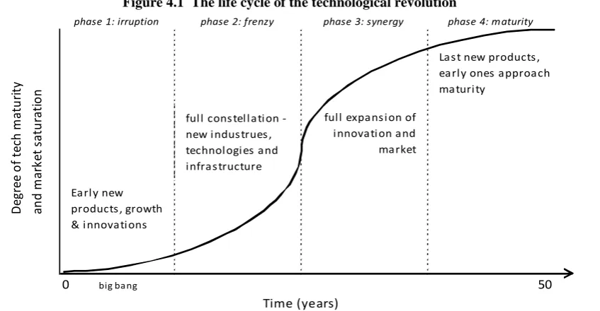
[image:13.595.93.517.157.377.2]She has identified four phases and a turning point in each technological revolution. The first phase is irruption: a time for technology; the second phase is frenzy: a time for finance; next comes the turning point: rethinking and rerouting development; the third phase is synergy: a time for production; the final phase is maturity: a time for questioning complacency. A simplified diagram of the model is set out in figure 4.1. The turning point is at the end of phase 2 and the beginning of phase 3.
Figure 4.1 The life cycle of the technological revolution
0 big bang 50
D
eg
re
e
o
f
te
ch
m
at
u
ri
ty
an
d
m
ark
et
s
at
u
ra
ti
o
n
full constellation - new industrues, technologies and infrastructure
full expansion of innovation and market
Early new products, growth & innovations
Time (years)
phase 1: irruption phase 2: frenzy phase 3: synergy phase 4: maturity
Last new products, early ones approach maturity
Further each revolution had or has a key factor which Perez describes as „a specific input which plays the role of the low cost key factor‟ which became widely available. For example as she says, „it is only in 1971, with the microprocessor, that the vast new potential of cheap microelectronics is made visible.‟ Perez says that it has often been suggested that the next technological revolution will be formed - arguably as a revolution in the 2030s - from the combination of biotechnology, bioelectronics and nanotechnology - in which we would identify in particular environmental requirements. Perez believes that what would make it revolutionary is a low cost factor „that would make it cheap to harness the forces of life and the power hidden in the infinitely small‟ but that this is still unpredictable. She does see meeting the environmental challenges as an important condition favouring the acceptance of significant changes in policy and potentially playing a crucial role in stimulating innovation.
Perez has identified two ways in which her model might apply to follower countries. On the one hand she identifies a final phase in the cycle of diffusion of a technological revolution in which development of mature technologies spreads to peripheral countries. On the other hand she says that follower countries can make significant progress in the early stage of a new technological revolution and in this connection says that „a key feature of the current Information Age is the establishment of a globalized economy,‟ where „the spreading of both production and trade networks across core and peripheral countries began from the early installation period‟ and suggests that „this feature is likely to distinguish this surge from all previous ones in terms of the rhythm of propagation to non-core areas.‟ Perez distinguishes clearly between what can be termed maturity growth and the more positive catching up, reminiscent of Schumpeter‟s distinction between growth and development.
In analysing the modernisation of the whole productive structure of economies Perez identifies four different types of branch or sector namely: motive sectors which produces the key factor; carrier sectors which are those that make intensive use of the key factor, infrastructural sectors whose impact is felt in shaping and extending the market boundaries for all sectors and induced sectors whose development is both a consequence and complimentary to the growth of the carrier branches.
123
Perez has set out a description of the key elements of her approach in her 2002 book and in the large number of papers to be found on her web site. In this paper we will deal with the way in which the Perez approach might be applied to Ireland based on our survey of the data over the last 50 years. We discuss technological revolutions and how they impact on a follower or peripheral country. We see how well structural change in the Irish economy fits the Perez model. We consider the branches that Perez isolates in analysing the way in which technological revolutions develop across economies and identify these branches in the Irish case. We also mention the consequences of the different behaviour of financial and production capital.
5. DATA AND ANALYSIS
We now examine the statistics to establish the extent and nature of structural economic change in Ireland over the past fifty plus years. We use four time periods or phases to reflect the macro economic development since 1957. First a fifteen year period from 1957 which started from a very traditional agriculture and protected industry base with good overall growth reflecting for many the new policy approach of Whitaker‟s Economic Development and the Lemass Programmes for Economic Expansion. Then a further fifteen year period to 1986 with good initially but later poor overall growth when we had an oil crisis, a somewhat misguided Keynesian justified policy push for growth which took little account of the open nature of the Irish economy coupled with entry to the then European Community. Next, the ten year period to 1996 when we had a return to good growth following on social partner based policies coupled with rapid global growth but little response from employment. Finally, from 1997 to 2006, when we had a continuation of rapid GDP growth and rapid employment growth in the Celtic Tiger era but headed into fiscal instability and the global financial crisis.
From the perspective of the present paper we will examine how the structure of the economy changed over the entire period and the extent to which this change varied with the macro pattern. We will do this in two ways: first, by identifying the pattern of the growth by sector; and secondly, by outlining the contribution of different sectors to that growth which takes account of the initial size of the sectors.
We present constant price tables in previous years‟ prices for value added at detailed sectoral level for each of the time periods. In each of the tables a reference year is chosen and the results are shown in the prices of that year. Years for which input-output tables are available are convenient choices as reference years. We choose the latest year in the time period where input-output tables are available. Changing the reference year is very straightforward and it makes sense to think of the tables simply as a set of indices by sector (by dividing the gross value added of each sector and each year by the gross value added of the reference year). For this reason linking the four tables is also straightforward. Thus the four tables together comprise the longest, most detailed, up-to-date and consistent series of its type available for the Irish economy.
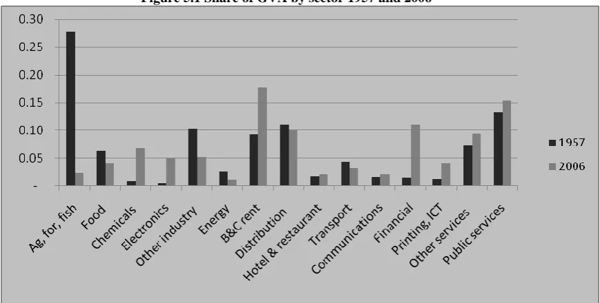
[image:14.595.90.525.542.762.2]We begin by presenting the Irish economy in 1957 and 2006 in Figure 5.1 so as to identify clearly the changes that have occurred in the last 50 years.
124
In summary: there is a substantial decline in agriculture; industry and energy together register a decrease and there is substantial shift within the aggregate from traditional to modern manufacturing; construction and financial services make up most of the fall in agriculture and there is some increase in other services and public services. The shift of the balance to services in the recent times has been remarked by a number of commentators; see for example [3] and McCarthy and O‟Leary [11].
Period 1 1957-1971
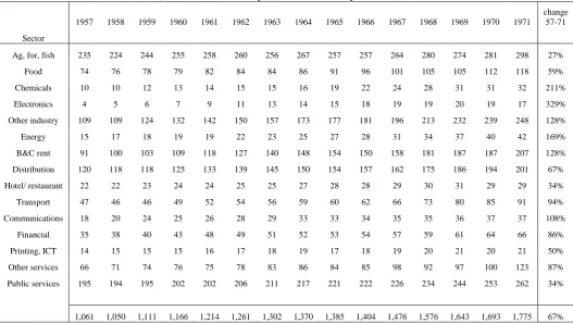
[image:15.595.41.569.232.529.2]Table 5.1 shows the GVA in constant previous years‟ prices at detailed sectoral level, for 1957 to 1971, referenced to 1969 prices. GDP at constant prices is shown at the end of the table and the percentage change over the fifteen years is given in the last column.
Table 5.1 Gross Value Added by sector of origin at constant market prices (chain-linked annually and referenced to year 1969)
1957 1958 1959 1960 1961 1962 1963 1964 1965 1966 1967 1968 1969 1970 1971
change 57-71
Sector
Ag, for, fish 235 224 244 255 258 260 256 267 257 257 264 280 274 281 298 27%
Food 74 76 78 79 82 84 84 86 91 96 101 105 105 112 118 59%
Chemicals 10 10 12 13 14 15 15 16 19 22 24 28 31 31 32 211%
Electronics 4 5 6 7 9 11 13 14 15 18 19 19 20 19 17 329%
Other industry 109 109 124 132 142 150 157 173 177 181 196 213 232 239 248 128%
Energy 15 17 18 19 19 22 23 25 27 28 31 34 37 40 42 169%
B&C rent 91 100 103 109 118 127 140 148 154 150 158 181 187 187 207 128%
Distribution 120 118 118 125 133 139 145 150 154 157 162 175 186 194 201 67%
Hotel/ restaurant 22 22 23 24 24 25 25 27 28 28 29 30 31 29 29 34%
Transport 47 46 46 49 52 54 56 59 60 62 66 73 80 85 91 94%
Communications 18 20 24 25 26 28 29 33 33 34 35 35 36 37 37 108%
Financial 35 38 40 43 48 49 51 52 53 54 57 59 61 64 66 86%
Printing, ICT 14 15 15 15 16 17 18 19 17 18 19 20 21 20 21 50%
Other services 66 71 74 76 75 78 83 86 84 85 98 92 97 100 123 87%
Public services 195 194 195 202 202 206 211 217 221 222 226 234 244 253 262 34%
1,061 1,050 1,111 1,166 1,214 1,261 1,302 1,370 1,385 1,404 1,476 1,576 1,643 1,693 1,775 67%
The table shows that the economy grew by 67% in the fourteen years. This is an average of 3.7% GDP growth per year. The growth from 1960 to 1971 is 52%. This compares well with table 7.1 of the Statistical Yearbook of Ireland 2004 where GDP growth over the same period is 55%. Our table indicates that the most sustained growth occurred in the period 1959-62 with growth rates ranging from 4% to 6%. Moderate growth occurs for other years except 1968 which peaks again to 7%. In these well performing years, it is other industry and B&C and real estate that contribute most significantly to this growth.
Agriculture holds a leading share of the total GVA for each year, but is the worst performing sector in terms of year-on-year growth. Conversely the volume of chemicals and electronics (office equipment) rise significantly in this period but have a small share of total GVA. It is interesting that these two hi-tech sectors already in the period 1957-71 are showing signs of their future promise. It is a feature of these industries to have a high value added to inputs ratio. This feature has the potential for rapid growth and is evident even when their relative significance is low.
125
to 24% of the total GDP. This is evidence of the development of Ireland‟s industrial base in the Lemass years in the periods of the first and second programmes for economic expansion in 1958. Increase in GVA of public services including health and education is lower than most other sectors. As public services are non-market, the GVA for this sector is calculated as its expenditure on goods and services plus compensation of employees. The series tells us that there was no real increase in public services employment numbers.
We consider also how much each sector contributes to growth of the whole economy. We measure a sector‟s contribution to the growth rate as the difference between that sector‟s contribution to a given year‟s GVA and its contribution to the GVA in the previous year divided by the total GVA of the previous year. Thus if Cit represents the GVA for sector i, in year t, and Gt the total GVA for the whole
economy in year t,we consider the factors,
(Cit - C i
t-1 )/ Gt-1
for all i, where each measure of GVA is in constant prices.
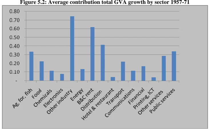
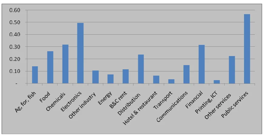
[image:16.595.114.482.293.519.2]The chart below shows the average contribution to GVA measured over each year from 1957 to 1971
Figure 5.2: Average contribution total GVA growth by sector 1957-71
We stated above that the average growth of the whole economy is 3.7% per year. Figure 5.2 tells us, for instance, that on average .74 of this growth is due to the „other industry‟ sector.
Apart from this sector, it is the relatively large sectors (including agriculture), throughout the full time period, that contribute most to growth. This is as one would expect when development is relatively even across the economy. This set of data is therefore not remarkable. In fact no real shift in structure is emerging. In hindsight, we notice the growth of the chemicals and hi-tech sector. But these are as yet fledgling industries. A commentator in 1972 is likely to have remarked that the analysis and frank self-assessment at the end of the 1950‟s led to policy decisions that opened up the economy and incentivised industrial development - thus the growth in the „other industry‟ sector comprising of clothing, building materials, furniture, etc. Further, although many of the policy decisions following the first economic programme for economic development were aimed at increasing agricultural output, through lowering of barriers to trade, the effect on agricultural development appears to have been negligible.
Period 2 1972-1986
126
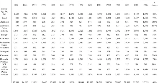
Table 5.2 GVA in constant prices for the years 1972-1986 chain linked annually and referenced to 1985 (€m).
1972 1973 1974 1975 1976 1977 1978 1979 1980 1981 1982 1983 1984 1985 1986
% change
Sector Ag, for,
fish 1,635 1,586 1,705 1,891 1,683 1,847 1,876 1,646 1,768 1,690 1,891 1,906 2,174 2,139 1,970 20%
Food 848 986 1,010 972 1,027 1,056 1,140 1,230 1,181 1,201 1,234 1,246 1,338 1,437 1,503 77%
Chemicals 227 279 317 278 353 392 524 627 571 662 632 735 831 996 1,059 366%
Electronics 195 234 258 222 285 421 453 497 550 696 801 977 1,228 1,391 1,551 694%
Other
industry 1,549 1,556 1,626 1,530 1,642 1,721 1,830 2,021 1,885 1,886 1,793 1,742 1,849 1,804 1,756 13%
Energy 373 368 372 352 373 390 433 486 465 507 512 518 559 612 561 50%
B&C rent 2,047 2,064 2,079 2,092 2,128 2,211 2,334 2,536 2,646 2,718 2,655 2,568 2,423 2,311 2,247 10%
Distribution 1,907 2,143 2,177 1,936 1,992 2,175 2,412 2,487 2,641 2,667 2,587 2,449 2,426 2,495 2,396 26% Hotel/
restaurant 331 368 392 384 365 403 457 474 456 436 427 431 467 480 479 45%
Transport 659 703 639 711 729 734 741 738 729 725 728 719 716 728 735 11%
Commun 185 185 218 255 266 299 320 370 399 419 403 453 497 518 568 206%
Financial 1,020 1,089 1,159 1,231 1,303 1,371 1,441 1,511 1,584 1,654 1,678 1,702 1,723 1,746 1,772 74% Printing,
ICT 185 194 194 185 193 192 208 234 232 234 220 210 227 234 249 34%
Other
services 458 485 476 432 500 524 658 672 766 788 802 962 1,036 1,136 1,049 129%
Public
services 2,835 2,953 3,107 3,309 3,379 3,444 3,581 3,730 3,874 3,930 4,024 3,957 4,048 4,103 4,192 48%
13,999 14,693 15,191 15,467 15,850 16,947 18,098 19,004 19,853 20,368 20,870 20,862 21,898 22,569 22,595 61%
Table 5.2 shows that the economy increased by 61% in volume terms in the period 1972 to 1986, with an average of 3.4% annual growth. This agrees with the growth in GVA between 1972 and 1986 to be seen on the CSO‟s historical series of national accounts available on the CSO website. The performance is however very uneven over the years. There is a very healthy period between 1976 and 1980 with an average of 6% growth per year. This is followed by low growth of little over 2% per annum with negative growth in 1983 and almost zero growth in 1986.
We see that not all sectors have performed equally well. Agriculture, forestry and fishing increased by just 20% in these years. Transport, consisting mainly of CIE and Aer Lingus as well as freight is another poor performing sector with growth rate of just under 1% per year over the 14-year span (signifying further cutbacks in rail and bus services after the initial line closures in 1958-62).
127
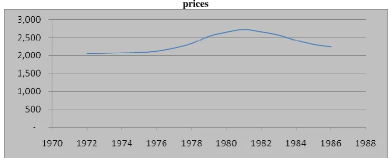
Figure 5.3: Value of real output of construction and rental services in €000 referenced to 1985 prices
In the manufacturing industry sector, the „other industry‟ sector has performed quite poorly. This sector was starting from a high base, as we noted before. It is primarily non-food traditional manufacturing whose development was quite marked in the previous period. The growth of this sector, however, was not sustained and many of the traditional industry types were disappearing in the 1971-1986 period. Leather and footwear, car manufacturing, shipbuilding and some of the textile industries are all industries which had over 75% less employees at the end of this period than at the beginning. This could partly be attributed to stronger competition from abroad to Ireland's relatively small-scale firms following Ireland‟s accession into the EC.
On the other hand, the food sector maintained a steady increase of 4% per year. It appears to reflect a move towards softer industries. Developing the point in the previous paragraph, it may be also that Ireland‟s membership of the EC has opened up markets in the food industry but not in other heavier traditional industries. It suggests also that Ireland is perhaps getting further value added from agricultural produce – that although the growth rate of agriculture since the late 1950s is rather small, the combined agri-food sector begins by the mid-seventies to modernise. See for instance Brendan Riordan [17].
There are some positive comments to be made of the period. The communication sector grows from €181m to €568m, in 1985 prices, as a result of the extension of telephones to all households in the country. This is further evidence of expenditure on capital programmes, which may have borne fruit at a later time. Energy provision also increases by 50% over the 14 years.
Of particular interest are two sectors that are to have such an important effect on the volume of GDP growth in later years – namely chemicals and electronics (office equipment). These industries are grouped along with reproduction of recorded media, in the current national accounts under the heading of modern industries and have a particular importance in our discussion of the Perez model. Chemicals increased by over 350% and electronics by nearly 700%.6 In the 14 year period these two sectors have moved from having a 4% to 10% share of total GVA. The value added for these sectors increases most spectacularly in the years after 1982, a time of economic depression for the country as a whole. We see here the success of policy decisions for the economy, particularly the decision by the IDA as early as 1972 to focus its attention on chemicals, electronics and other hi-tech industries.
As in the previous discussion we consider how much each sector contributes to growth of the whole economy. Figure 5.4 shows the average contribution by sector to the growth. Factors influencing the height of each bar are the growth rate of the sector and the share of the economy that that sector maintains.
6
128
Figure 5.4 Average annual contribution to total GVA growth by sector 1972-86
Figure 5.4 is different from the equivalent chart in the previous period. Very definite patterns are emerging. In the current case financial services, other services, public services, chemicals and electronics are the dominant sectors whereas agriculture and other industry sector have been relegated to the background.
The significance of public services (now the largest sector) is notable. The increase is due to expansion in numbers which may have come about after Ireland‟s entry into the EU. Education is also a factor since the full implementation of free second level education.
The financial and other services sectors contribute significantly to GVA growth between 1972 and 1986. This suggests a move from primary and secondary to tertiary industries. Some of the weight of economic growth moves from manufacturing to services. In this period, service type activities and financial services are on the whole domestically based. The growth of these sectors in a time of economic recession does however provide a sound platform for building a substantial export driven services in coming years.
The dominance of chemicals and electronics represents a significant change in the manufacturing sector. Looking again at table 5.2, food products and other industry are both larger than either chemicals or electronics throughout the period (except 1986, where electronics are greater than food products). It is clear however that traditional manufacturing is now being challenged by modern, hi-tech industries with phenomenal average annual growth of 12% and 16%, for, respectively, chemicals and electronics, over this period.
In figure 5.3, therefore, we witness a sizable shift in the structural composition of the economy. We see the rise of chemical and electronic production, which are for the most part foreign-owned. We see the corresponding decline of importance of traditional domestic manufacturing industries and agriculture. Service industries maintain an important value to the economy. There is evidence too of an element of capital formation.
Period 3 1987-1996
129
Table 5.3 GVA in constant prices for the years 1987-96 chain linked annually and referenced to 1990 (€m).
1987 1988 1989 1990 1991 1992 1993 1994 1995 1996
change 87-96
Sector
Ag, for, fish
2,397 2,526 2,560 2,958 2,891 3,130 2,876 2,807 2,747 3,081 29%
Food 2,137 2,240 2,364 2,460 2,632 2,847 2,876 3,114 2,955 3,056 43%
Chemicals 1,155 1,194 1,349 1,558 1,740 2,062 2,134 2,536 2,972 3,500 203%
Electronics 1,527 1,955 2,329 2,322 1,996 2,291 2,282 2,791 3,847 3,897 155%
Other industry 1,857 1,963 2,173 2,218 2,271 2,231 2,307 2,396 2,471 2,655 43%
Energy 489 502 536 577 568 584 602 624 566
605 24%
B&C rent 2,840 2,789 2,907 3,178 3,189 3,219 3,309 3,511 3,730 4,094 44%
Distribution 2,550 2,657 3,123 3,929 3,868 3,232 3,608 3,554 4,101 5,003 96% Hotel & restaurant 585 627 671 693 693 738 784 850 927 1,024 75%
Transport 962 963 1,067 1,114 1,145 1,150 1,136 1,167 1,145 1,143 19%
Communications 719 765 809 856 901 958 989 1,081 1,141 1,262 75%
Financial 1,996 2,077 2,134 2,232 2,287 2,320 2,328 2,359 2,424 2,484 24%
Printing, ICT 335 380 414 424 575 601 612 614 598
627 87%
Other services 2,919 2,615 2,384 2,673 2,883 3,462 3,425 4,087 3,998 5,411 85%
Public services 5,186 5,236 5,313 5,461 5,471 5,525 5,644 5,633 5,685 5,742 11%
27,716 28,416 30,059 33,049 33,465 34,447 35,275 37,228 40,880 44,643 61%
Table 5.3 shows that the economy increased by 61% between 1987 and 1996. This is an average of 5.4% per annum. The growth is rather uneven. 1990, 1995 and 1996 had growth of over 9% whereas in 1988, 1991 and 1993 growth is less than 3%. In the years of very high growth, the distribution sector contributes significantly to the growth. Table A in the introduction of NIE2006 shows personal consumption of goods and services in constant prices from 1970 to 2006 in constant prices. These years of strong growth also showed higher than usual personal consumption.
Growth in agriculture is 29% for the full period. Half of this growth actually occurs between 1995 and 1996 and is due mainly to changes in the method of paying farm subsidies. Thus the growth in agriculture is not very strong.
GVA of public services increased by just 11% in this period, with growth hovering around zero from 1989 to 1995. This may illustrate efforts by the governments at the time to deal with Ireland‟s large foreign debt by cutting back on public spending. Public services were the largest contributors to growth in the last period. Here public services contribute very little to GVA growth rates. This illustrates, whether deliberately or not, a Keynesian type relationship between government spending and the economy.
The building and construction and rent of dwellings sector continues, at first, the downward trend exhibited in the previous period but picks up in 1988. From 1993 to 1996 growth averages 7.3% per annum. The growth over the period of building alone is 75%.
130
Figure 5.4 Average annual contributions to total GVA growth by sector 1987-96
Figure 5.4 shows the contribution to GVA by sector averaged over the years 1987-96. Chemicals and electronics dominate industry as before. The most remarkable sector is distribution, which has come to play a very central role in its contribution to growth in the economy. This is an important shift in the economy, representing to some extent the start of an era of consumption.
Period 4 1997-2006