Multi Objective Dynamic Economic Dispatch With Cubic Cost Functions

(1)

Multi Objective Dynamic Economic Dispatch With Cubic Cost Functions

M. Manjusha

1

_{, Dr. S. Farook}

2

1

_{P.G. Scholar, Dept. of Electrical and Electronics Engineering,}

2

_{Associate Professor, Dept. of Electrical and Electronics Engineering,}

12

_{Sree Vidyanikethan College of Engineering, Tirupati, Andhra Pradesh, India.}

---***---

Abstract -

Economic dispatch (ED) is the most important problem in the power system operation and control. Optimization of power system operation is generally assumed to be a smooth static economic dispatch (SED) modeled as a quadratic cost function. However this model makes many assumptions which are impractical to real systems. Consideration of such assumptions in ED formulation leads to the dynamic economic dispatch (DED) formulation. When more than two objectives are taken in to consideration a multi objective dynamic economic dispatch (MODED) is formed. The MODED has been considered on a quadratic cost function which is less accurate. In this paper we consider the higher order cost functions for example cubic order cost functions to model MODED problem. This higher order cost functions are more accurate and realistic than the traditional quadratic cost functions. In this paper unit commitment (UC) also considered along with MODED problem with four objectives. Dynamic programming method was used for UC and Lagrange's method was used for MODED.

Key Words

:

Power system optimization, economic dispatch, multi objective dynamic economic dispatch problem, unit commitment, valve point effect loading, Lagrange’s method and dynamic programming method.

1. INTRODUCTION

Today the main aim of electric power utilities is to provide high-quality reliable power supply to the consumers at the lowest possible cost while operating to meet the limits and constraints imposed on the generating units and environmental considerations. These constraints formulates the economic load dispatch (ELD) problem for finding the optimal combination of the output power of all the online generating units that minimizes the total fuel cost while satisfying an equality constraints and a set of inequality constraints. Economic dispatch is the short term determination of the optimal output of the generators, to meet the system load, at the lowest possible cost, subjected to different transmission and operational constraints.

DED problem is one of the most important problem which must be taken into consideration in power systems planning and operation. DED is aimed at planning the power output for each devoted generator unit in such a way that the operating cost is minimized and simultaneously, matching the load demand, operating limits and above all maintaining the system stability.

The Thermal, Emissions, reserve cost functions and Transmission Loss cost functions when considered individually, results in a Single Objective DED (SODED).Where more than two objectives are taken into consideration, a MODED problem results. The solution accuracy of economic dispatch problems is associated with the accuracy of the fuel cost curve parameters. In most studies, the generation cost function is considered to be quadratic function, but a cubic cost function more closely conforms to the generation cost. Therefore, the use of a cubic cost function leads to more accurate modeling of power plant costs.

(2)

2. MATHEMATICAL MODELLING

2.1. UNIT COMMITMENT PROBLEM FORMULATION

The objective function of UC problem is the minimization of the total cost which is the sum of the fuel cost and the start up cost of individual units for the given period subject to various constraints. Mathematically, the UC problem model can be formulated as [6]

             



( ₍(₁)) ₎

min

) 1 ( 1 1 i it

i i T t N i it

t _SUC _U

t p F U F Eq. 1

where F_t is the total operating cost in $, F_i(p_i(t)) is the fuel cost of unit i at hour t p_i(t) is the output power of ith unit at hour t,

it

U is the on/off status of ith unit at hour t.

The major component of the operating cost, for thermal units, is the power production cost of the committed units. This can be calculated using the economic dispatch problem. In this paper MODED with four objectives was considered.

2.2. MODED PROBLEM FORMULATION

The proposed MODED problem is to minimize four objective functions namely fuel cost with valve point effect, reserve cost, transmission losses cost and emission, while satisfying a set of equality and inequality constraints. The mathematical formulation of this MODED problem is described as follows.

Fuel cost function -

The cost function is generally considered to be a square (Quadratic) cost function . However, a cubic cost function is more appropriate and accurate. So, the proposed total generation cost can be expressed as follows:

) (

min 3 2

1 1 i i i i i i i N i i N i

i p a p b p c p d

F

F 







  

 

Eq. 2

where

F - Total fuel cost )

( _i

i p

F - Fuel cost of the

i

th generator

i

p - real power generation of unit i

i i i i b c d

a , , , - cost coefficients

N - Total number of generators

Thermal power plants have multiple steam valves. To accurately evaluate the fuel cost function, the valve point effect loading is considered as follows:

(3)

F -Total fuel cost with valve point effect

i i f

e, -valve point effect coefficients of unit i

Power plant spinning reserve cost function -

Plants should have enough spinning reserve to provide energy for the customers without interruption. This reserve provides cost for the system. The determination of spinning reserve values to minimize the total reserve cost function is one of the main objective in power system operation. Therefore,

) (

min 2

1 1

cos ri i ri i ri N

i i N

i i

t FR R a R b R c

FR 







 

 

Eq. 4

where FR_cos_t is the total reserve cost of the whole system, R_i is the reserve for the ith unit and a_ri,b_ri,c_ri are the coefficients of

the reserve cost of the th

i generator.

Transmission line losses cost function -

Generally the generating centers and the connected load exist in geographically distributed scenario. So, the transmission network losses must be taken into account to achieve true economic dispatch. Network loss is a function of power injection at each node. Where the real power system transmission loss, PL, is expressed using B- coefficients as follows:

00 1

0

1 1

B P B P B P

P _i

n

i i j

ij n

i n

j i

L 

 







  

Eq. 5

Where i is the number of generators , j is the number of buses in the system, Bij is the ijth element of the loss coefficient Square

matrix, B₀_i is the ith element of the loss coefficient matrix and B₀₀ is the constant loss coefficient .

The cost of transmission line losses between plants are accounted with the actual fuel cost function by using a price factor g .This factor is defined as the ratio between the fuel cost at its maximum power output to the maximum power output .That is for this multi objective case

max , 1

max , )

(

i N

i i

p p F

g





 Eq. 6 Thus, the cost function for the losses at a

particular time becomes

) ( )

(

1

, L

N

i i i

L g p

p

F





 Eq. 7

Emission dispatch formulation -

The emission function of economic load dispatch problem is defined as follows [3]:

i i i i i i i

ij P P P

p

E( ) 3 2  Eq. 8

(4)

The proposed objective function -

The proposed MODED problem can be mathematically formulated as follows [1], [2]:

)}) ( { } ) ( { min( min 2 cos , 1 ij t i L vp p E W FR p F F W

F    

Eq. 9

2 1,W

W are non-negative weights used to make tradeoff between emission security and total fuel cost such that W₁W₂1 .

2.3. CONSTRAINTS

system power balance -

() ()

1

t p t p

U _i _d

N

i

i 





_{Eq. 10}

where p_d(t) is the power demand at ithinterval.

Spinning Reserve Constraints -

The sum of the maximum power generating capacities of all the committed units at a time instant should be at least equal to the sum of the known power demand and minimum spinning reserve requirement at that time instant [8], i.e.

t d i

N

i

itp p t R

U  





) (

(max)

1 _{Eq. 11}

where pi(max) is the maximum power that can be generated by unit i and Rt is the minimum spinning reserve requirement at time

t.

Generation Limit Constraints

-0 0 ) ( 1 ) ( _(max) (min)      it i it i i i whenU t p whenU p t p p Eq. 12

where pi(min) and pi(max) represents the minimum and maximum generation limits of thermal units.

Unit Minimum up/down Time Constraints -

















0

0 ) 1 ( ) 1 ( ) 1 ( ) 1 (             t i it off i off t i it t i on i on t i U U T X U U T X Eq. 13

where on t i

X ₍₎and X_ioff₍_t₎ is the time duration for unit i has been on and off respectively at hour t.

Ramp Rate Limits -

p_i(t)p_i(t1)UR_i

i i

i t p t DR

p( 1) () _{Eq. 14}

(5)

3. MODED BY LAGRANGE'S METHOD

The MODED problem is solved using Lagrange’s method by introduction of the Lagrange’s variables λ,



and formulation of a Lagrange’s function:

) (

1 1

SP R p

p p F

L

N

i i loss

d N

i i

T     





 

 

Eq. 15

where , are the Lagrange multipliers, R_i is the reserve capacity of ith generator, SP is the spinning reserve.

)) max( , * 1 . 0

max( load pi

SP

Algorithm for this method is as follows: Step 1:- Read the data.

Step 2:- Calculate the

max 1

max₎

(

i N

i i

i p

p F

g



 

Step 3:-Equation 0 



i

p L

is solved and k i

p was determined. Check the obtained vector is fit to the constraints.

Step 4:- Equation 0 



i

R L

is solved and R_i was determined and check for the spinning reserve constraints.

Step 5:- Calculate the losses using equation(5).

Step 6:- Equation 0

   L

is solved and k 0



 was calculated.

Step 7:- Check the condition  k 

Step 8:- If the condition is fulfilled the calculations are stopped, if not, improve the value of _k_→_k1_.

Step 9:- Calculations of the improved values of _ k1 i k

i p

p and repeat the steps 3,4,5and 6.

Step 10:- Iterations were continued until the condition 



k 



_{was satisfied.}

Step 11:- Optimal solution is used to calculate the total production cost.

4. UC BY DYNAMIC PROGRAMMING METHOD

(6)

2) Well-established theory;

3) Fast execution time.

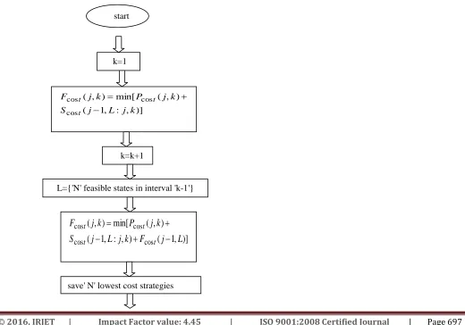
This model is based on the priority list method but accounts for start-up and no-load costs, and minimum up and down times. A priority list [13] contains all state combinations of generators. The combinations or states are then listed from highest maximum net output power to lowest. When given the total load demand for any particular hour the list is used to determine which combinations are feasible. The feasible states include all combinations, which have a maximum net output power greater than or equal to the load demand. The costs of all feasible states are calculated and the lowest cost combination is stored. Usually in the forward-dynamic programming method the cost function is assumed to be linear, however, in this case the function is a cubic. For any given state, the cost for that state is given by the following expression:

F(P) = No-load cost + Incremental fuel cost × Power + Constraint costs.

[image:6.612.39.559.378.742.2] [image:6.612.47.275.383.733.2]

In addition to thermal constraints, several other constraints must be considered when choosing generator combinations. The recursive algorithm is used to compute the minimum cost in hours 't' with feasible state 'L' is [10]:

Fig. 1 represents the flow chart for the unit commitment problem with dynamic programming method. ( 1, )]

) , : , 1 ( ) , ( min[ ) , ( cos cos cos cos L j F k j L j S k j P k j F t t t t      start

k=1 )] , : , 1 ( ) , ( min[ ) , ( cos cos cos k j L j S k j P k j F t t t   

k=k+1

L={'N' feasible states in interval 'k-1'}

)]

,

1 (

)

,

:

,

1 (

)

,

(

min[

)

,

(

cos cos cos cos

L

j

F

k

j

L

j

S

k

j

P

k

j

F

t t t t











(7)

Fig – 1: Flowchart for UC by dynamic programming method

5. SIMULATION RESULTS OF MODED WITH UC

[image:7.612.38.438.356.713.2]

The four generator system is represented by fuel cost with valve point effect, reserve coefficients, emission coefficients and real power limits as given in Table 1.Unit characteristics and load characteristics were given in Table 2 and 3. The problem is solved in Mat lab environment. The Lagrange’s method is used to obtain the solution of the dispatch problem. Dynamic programming method is used for UC problem. The solution of this problem for 8 hours is shown in Table 4.

Table 1. Characteristics of the four unit system

PARAMETERS Gen-1 Gen-2 Gen-3 Gen-4

a($) 4.1*10^-8 8.1*10^-8 8.1*10^-7 8.2*10^-8

b($/MW) 0.00028 0.00056 0.00056 0.00056

c($/MW^2) 0.0081 0.0081 0.0081 0.0081

d($/MW^3) 35 30.9 30.9 30.9

e 300 200 200 200

f 0.035 0.042 0.042 0.042



75 63 63 63



-5.76 -5.46 -5.46 -5.46



0.09 0.093 0.093 0.092

ri

a

45 52 52 52

ri

b

0.09 0.12 0.12 0.12

k=last hour

Trace optimal schedule

(8)

ri

c

0.0044 0.0056 0.0056 0.0056

min

pg

0 0 0 60

max

pg

680 360 360 400

Table 2. Unit characteristics

Unit No load cost Rs/h

Full load avg. cost Rs/MWh

Initial condition

Incremental heat rate Btu/KWh

Min up time

Min down time

Cold start up cost

Hot start up cost

1 213 23.54 -5 10440 4 2 350 150

2 585.62 20.34 8 9000 5 3 400 170

3 684.74 19.74 8 8730 5 4 1100 500

4 252 28 -6 11900 1 1 0.02 0

Table 3.Load demand for three units.

Hour

1

2

3

4

5

6

7

8

9

10

11

12 Demand 450 1530 600 540

400 1280 290 1500 1100 1221 390 490

Hour

13

14

15

16

17

18

19

20

21

22

23

24 Demand 450 569

890 1000 980 1100 560 452

780

600 400 395

Table 4. UC Results for the 4 generator test system

Hour Demand

Unit Status

Power generation

Producti

on cost

Transiti

on

cost+

previou

s state

cost

Total

cost

G1

G2

G3 G4

Pg1

Pg2

Pg3

Pg4

1

600

0

1

0

1

0

310

0

304.6

737.7

0

737.7

(9)

3 1000

1

0

1

607.

6

0

400

874.2 1532.4

2406.6

4

900

1

0

1

505.

1

0

400

994.8 2406.6

3401.4

5

800

1

0

1

408.

6

0

394.7 1163.2

3401.4

4564.6

6 1050

1

0

1

659

0

400

838.7 4564.6

5403.3

7 1000

1

0

1

607.

6

0

400

874.2 5403.3

6277.5

8

700

1

0

1

357.

9

0

344.9

959.7 6277.5

7237.1

6. CONCLUSION

The multi objective dynamic economic dispatch problem with four objectives (fuel cost including with valve point effect, reserve cost, losses cost and emission) including unit commitment was formulated. The Lagrange’s algorithm is developed for the solution of the MODED problem, dynamic programming method for UC.

REFERENCES

[1] Boubakeur Hadji, Belkacem Mahdad, Kamel Srairi and Nabil Mancer, “Multi-objective Economic Emission Dispatch Solution Using Dance Bee Colony with Dynamic Step Size”, Elesiver , Energy Procedia, vol. 74, pp. 65–76, Aug. 2015.

[2] Moses Peter Musau, Nicodemus Odero Abungu, Cyrus Wabuge Wekesa. "Multi Objective Dynamic Economic Dispatch with Cubic Cost Functions," International Journal of Energy and Power Engineering. Vol. 4, No. 3, pp. 153-167, 2015.

[3] S Subramanian and S Ganesan. “A Simple Approach for Emission Constrained Economic Dispatch Problems” International Journal of Computer Applications Vol. 8, No. 11 pp39–45, October 2010.

[4] Haiwang Zhong; Qing Xia; Yang Wang; Chongqing Kang, "Dynamic Economic Dispatch Considering Transmission Losses Using Quadratically Constrained Quadratic Program Method," Power Systems, IEEE Transactions on , Vol.28, No.3, pp.2232-2241, Aug. 2013.

[5] http://www.sciencedirect.com/science, April 2015.

[6] A. J. Wood, and B. F. Wollenberg, Power generation, operation and control, 2nd ed., New York: John Wiley & Sons, 2nd ed.,2007.

[7] W. L. Snyder Jr., H. D. Powell Jr., and J. C. Rayburn, “Dynamic programming approach to unit commitment,” IEEE Transactions on Power Systems, vol. PWRS-2, no. 2, pp. 339-350, May 1987.

(10)

© 2016, IRJET | Impact Factor value: 4.45 | ISO 9001:2008 Certified Journal | Page 701 [9] N.P. Padhy,"Unit Commitment-a Bibliographical Survey," Power Systems, IEEE Transactions on, Vol. 19, No. 2, pp.

1196-1205, 2004.

[10] W. J. Hobbs, et. al., “An enhanced dynamic programming approach for unit commitment,” IEEE Trans. Power Syst., Vol. 3, No. 3, pp. 1201-1205, August 1988.

[11] C. C. Ping, L. C. Wen, and L. C. Chang, “Unit Commitment by Lagrangian Relaxation and Genetic Algorithms, ” IEEE Trans. Power Syst., Vol. 15, No. 2, pp. 707-714, May 2000.

[12] N.A Amoli et al “Solving Economic Dispatch Problem with Cubic Fuel Cost Function by Firefly Algorithm” Proceedings of the 8th International Conference on Technical and Physical Problems of Power Engineering, Ostfold University College Fredrikstad, Norway. pp 1-5, 5-7th September 2012.

[13] F. Benhamida, E N. Abdallah, A. H. Rashed, “Solving the Dynamic Economic Dispatch as Part of Unit commitment problem,” AMSE, Modeling General Physics and ElectricalApplications, Vol. 78, No. 5, pp. 49-63, 2005.

[14] R. M. Burns and C. A. Gibson, “Optimization of priority lists for a unit commitment program,” in Proc. IEEE Power Eng. Soc. Summer Meeting, 1975, Paper A 75 453-1.