A g e n e r a l i n s p e c ti o n a n d
o p p o r t u n i s ti c r e p l a c e m e n t p olicy
fo r o n e-c o m p o n e n t s y s t e m s of
v a ri a bl e q u a li ty
C a v al c a n t e , CAV, Lo p e s , R S a n d S c a rf, PA
h t t p :// dx. d oi.o r g / 1 0 . 1 0 1 6 /j. ejor. 2 0 1 7 . 1 0 . 0 3 2
T i t l e A g e n e r a l in s p e c tio n a n d o p p o r t u n i s ti c r e p l a c e m e n t p olicy fo r o n e-c o m p o n e n t s y s t e m s of v a ri a bl e q u a li ty
A u t h o r s C a v al c a n t e , CAV, Lo p e s , R S a n d S c a rf, PA
Typ e Ar ticl e
U RL T hi s v e r si o n is a v ail a bl e a t :
h t t p :// u sir. s alfo r d . a c . u k /i d/ e p ri n t/ 4 4 0 5 6 / P u b l i s h e d D a t e 2 0 1 8
U S IR is a d i gi t al c oll e c ti o n of t h e r e s e a r c h o u t p u t of t h e U n iv e r si ty of S alfo r d . W h e r e c o p y ri g h t p e r m i t s , f ull t e x t m a t e r i al h el d i n t h e r e p o si t o r y is m a d e f r e ely a v ail a bl e o nli n e a n d c a n b e r e a d , d o w nl o a d e d a n d c o pi e d fo r n o
n-c o m m e r n-ci al p r iv a t e s t u d y o r r e s e a r n-c h p u r p o s e s . Pl e a s e n-c h e n-c k t h e m a n u s n-c ri p t fo r a n y f u r t h e r c o p y ri g h t r e s t r i c ti o n s .
A general inspection and opportunistic replacement policy for
one-component systems of variable quality
C.A.V. Cavalcante, Universidade Federal de Pernambuco, Department of Engineering Management, Recife PE, CEP:50740-550, Brazil (email: [email protected])
R.S. Lopes, Universidade Federal de Pernambuco, Department of Engineering Management, Recife PE, CEP:50740-550, Brazil (email: [email protected])
P. A. Scarf*, Salford Business School, University of Salford, Manchester M5 4WT, UK (email: [email protected])
*corresponding author
Abstract: We model the influence of opportunities in a hybrid inspection and replacement policy. The base policy has two phases: an initial inspection phase in which the system is replaced if found defective; and a later wear-out phase that terminates with replacement and during which there is no inspection. The efficacy of inspection is modelled using the delay time concept. Onto this base model, we introduce events that arise at random and offer opportunities for cost-efficient replacement, and we investigate the efficacy of additional opportunistic replacements within the policy. Furthermore, replacements are considered to be heterogeneous and of variable quality. This is a natural policy for heterogeneous systems. Our analysis suggests that a policy extension that allows opportunities to be utilised offers benefit, in terms of cost-efficiency. This benefit is significant compared to those offered by age-based inspection or preventive replacement. In addition, opportunistic replacement may simplify maintenance planning.
Keywords: Maintenance modelling, reliability, delay time, mixtures.
1 BACKGROUND
Preventive maintenance is widely accepted as an effective way of reducing the total cost of ownership of industrial assets (Xia et. al 2015). Maintenance management of industrial systems consists mostly of a variety of maintenance strategies, such as preventive maintenance, corrective maintenance, inspections and so on (Lee and Cha, 2016; De Almeida et al., 2015). The main objectives of maintenance management are related to increasing the reliability and availability of systems and to reducing the cost of maintenance (Berrade et al., 2013; Zheng, et al., 2016).
constitute these technical systems (Dekker and Smeitink, 1991). However, opportunistic maintenance can be considered as distinct from grouped maintenance policies (Wildeman et al., 1997) that exploit similar interdependencies but which consider maintenance for groups of components or parts or sub-systems (Peng and Zhu, 2017). Grouped policies aim to optimise maintenance for each in the set of components (Vu et al., 2015), whereas opportunistic maintenance optimises maintenance for one or a few components using stoppages that arise due to others.
Also interesting is that opportunities might be considered in the context of inspection maintenance, modelled through the delay time concept of Christer (1999). This connection is not well developed in the literature and there are few articles that address it (Wang and Christer, 2003; Berrade et al., 2017). We build on this connection in this paper, developing a model that is more general than those researched to date.
For this new model, we develop expressions for the long run cost per unit time (Ross, 1996) or cost-rate. The models consider a single-component system that is periodically inspected up to age
K (and replaced if it is defective), replaced at opportunities after age S, and replaced preventively
at age T. Furthermore, components arise from a heterogeneous population (Scarf et al., 2009, Scarf and Cavalcante, 2010) in a way that represents variability in the quality of components or maintenance workmanship (e.g. between different, competing suppliers). The new policy is natural in these circumstances. Furthermore, because inspection has the function to reveal defects and as we are dealing with heterogeneous population, the larger is the proportion of weak components, the more important is the role of the inspection. The hybrid policy is a natural one in these circumstances as it has similarities to “burn-in” policies (Zhang et al., 2014). For the new policy we develop, we describe its behaviour over a range of model parameter settings that typically arise in practical applications.
The layout of this paper is as follows. First, we explicitly describe the system, the failure model, and the maintenance policy, and their assumptions. Cost-rates for the two policies are then developed and their respective graphical representations are illustrated. We analyse the cost-effectiveness of proposed policies by comparing the cost-rate resulting for policies that are special cases of the proposed policies. A numerical example illustrates the performance of the different policy variations for a set of cost and reliability parameters. We finish with concluding remarks.
2 THE MAINTENANCE POLICIES 2.1 Description of the technical system
In maintenance modelling, the first thing that we should observe is the potential for practical contribution of a proposed model. Thus, the process of the construction of a model should begin with the observation of engineering practice, including an analysis of the feasibility of application (Scarf, 1997). One may observe specific situations for which appropriate maintenance policies are limited. This is the case for maintenance of a system composed of components from a heterogeneous population, which as already stated arises in many different contexts and where there exist decision problems regarding, for example, supplier selection (Berrade et al., 2012), quality of maintenance (Scarf and Cavalcante, 2012), reliability (Castet and Saleh, 2010), and analysis of failure warranty data (Attardi et al., 2005; Lee et al., 2016).
(time to defect or fault arrival), arises from a mixture distribution FX( )t pF t1( ) (1 p F t) 2( ). Here, p is a mixing parameter, so that components arise from a mixed population of “weak” and “strong” sub-populations. F1 and F2 follow any increasing failure rate (IFR) distributions, for example, Weibull distributions with characteristic lives 1, 2and shape parameters 1, 2 1. We denote the corresponding density and reliability function by fX and FX. This notion of a mixed population of weak and strong components is a natural consideration in the context of the hybrid policy that we develop in this paper and define in section 2.2.
The system is a critical system so that failures are immediately revealed. Inspection on the other hand determines whether the system is good or defective. Replacement of the system corresponds to replacement of the component and renewal of the system. Events occur that provide opportunities for preventive replacement. Practically, these may arise in broadly two ways: those that are external to the system, such as temporary falls in demand; and those that arise in a multi-component system of which the system of interest is one part. In the latter, we assume the single component system is stochastically independent of the rest of the system, so that the failure process of the single component system is independent of that of the rest of the system. The rest of the system is conceptually a complex system for which stoppages (opportunities) arise according to a Poisson process with rate μ. External events are conceptually the same.
When the system is in the defective state, it continues to perform its operational function (e.g. a noisy but functioning bearing). The time in the defective state, H (the delay time) has density
( ) H
f h and distribution function FH( )h , and X and H are statistically independent. Opportunities are independent of X and H. At replacement, the system age is set to zero. Thus replacement is renewal, and throughout the paper replacement and renewal are synonymous. We will also use the terms component and system interchangeably.
2.2 The maintenance policies
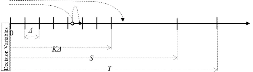
The principal policy is as follows. From new, the system is inspected every ∆ time units until K
[image:4.595.85.490.586.701.2]or a defect is found at inspection or a failure occurs, whichever occurs soonest. Inspections are perfect in that the true state of the system is revealed at inspection. Further if the system survives beyond age K, then inspection ceases, and the system is replaced on failure or at age T or at the first opportunity that arises after age S (S T ), whichever occurs soonest. Replacements are instantaneous. The policy has four decision variables: ∆, K, S, and T (Figure 1). The cost parameters are defined in Table 1, which shows the principal notation.
Figure 1. Graphical representation of the policy. A defect arises at ○ at age x leading to failure ● h
time units later; ▼ represents the arrival of an opportunity at time z. Table 1. Notation
Inspection interval
Δ
0
De
cisio
n
Va
riab
les
KΔ
K Number of inspections
S Age threshold for opportunistic replacement
T Age limit for preventive replacement
M In policy 2, M is such that S M
(.) X
F Time to defect arrival distribution
(.) H
F Delay time distribution
i
Weibull shape parameter for sub-population i
i
Weibull characteristic life for sub-population i p Mixing parameter
Reciprocal of the mean of the delay time distribution
Rate of arrival of opportunitiesI
C Cost of an inspection
R
C Cost of a replacement of a defective component and cost of a preventive
replacement of a component at age T
F
C Cost of a replacement of a failed component
O
C Cost of a preventive replacement at an opportunity, CO CR CF
( k)
E U Expected cost of a renewal cycle for policy k, k 1, 2.
( k)
E V Expected length of a renewal cycle for policy k, k 1, 2.
,
k
C Cost-rate for policy k , k 1, 2
The innovation of this model is the consideration of the age threshold for opportunistic replacement S, whereby replacement is carried out at opportunities that arise during the wear-out phase (K, ]T . In this way, the policy takes greater care in the initial life of an equipment and then in mid-life utilises opportunities for more cost-effective replacement. We call this policy 1 and study this in detail in the paper.
We also study a special case of policy 1 for which T K , so that inspection is carried out through the entire life of the system, and S M
(0
M
K
)
, so that opportunities that arise after the M-th inspection are utilised for replacement. This policy has three decision variables, ∆, K, and M. We call this policy 2.Many other special cases of the principal policy arise. If S T, then we have the policy proposed by Scarf et al.(2009), and opportunities are not utilised. If K 0, then there is no inspection phase, and policy corresponds to opportunistic age based replacement (Scarf and Deara, 1998). If K 0 and S T , then the policy is age based replacement with age replacement limit T
(Barlow and Proschan, 1966). With, K 0 and T we have the opportunistic replacement policy (Dagpunar, 1996). If
(
K
,
S
T
)
then we have a pure inspection policy; this is the single component delay time model (Christer, 1987).determine the relative efficiency of inspection and non-inspection, or the relative cost-efficiency of a policy with an ultimate age limit for replacement
( , , , )
K
S T
and without( , , ,
K
S T
)
.The motivation for policy 2 is related to application in practice. The management of policy 2 is relatively simple, because it demands only the monitoring of the number of inspections since new, so that if an opportunity arises after the M-thinspection but before the final inspection at K it can
be utilised. By definition, policy 1 must have a lower cost-rate that policy 2 (at their respective optima). However, the simpler management of policy 2 (or any other special case policy for that matter) may compensate for the increased cost.
3 CALCULATION OF THE COST-RATE 3.1 Policy 1
To develop the cost-rate, we calculate the probabilities of all renewal scenarios. The policy has four decision variables: ∆, the inspection interval; K, the number of inspections in the inspection phase;
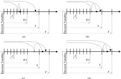
[image:6.595.106.504.385.643.2]S, the age threshold for opportunistic replacement; T, the age limit for replacement. The policy is fully defined in section 2.2. We can characterize the events related to four different kinds of renewal scenarios: scenarios related with failure (Figure 2); scenarios related with preventive replacement (Figure 3), and finally, scenarios related with opportunities (Figure 4).
Figure 2. Graphical representation of renewal on failure: (a) during the inspection phase, (b) in the wear out phase prior to the opportunity threshold S, (c) after the opportunity but before an opportunity arises and where the defect arises before S, and (d) the same but defect arising after S.
○ denotes a defect arrival, ● denotes a failure. and ▼ the arrival of an opportunity. Δ
KΔ
De
cisio
n
Va
riab
les
S
T
(a)
T Δ
KΔ
De
cisio
n
Va
riab
les
S
(b)
S Δ
KΔ
De
cisio
n
Va
riab
les
T
(c)
S Δ
KΔ
De
cisio
n
Va
riab
les
T
Figure 3. Graphical representation of renewal at preventive replacement: (a) at inspection, (b) at T
with defect arising before S, (c) at T with defect arising after S and before T, and (d) at T with no defect arising before T.
Figure 4. Graphical representation of renewal at an opportunity: (a) where the notional failure occurs after S and before T, and (b) where the notional failure occurs after T.
A failure can occur in four different ways, wherein there is renewal on failure: during the inspection phase [0,K] (Figure 2a); after the inspection phase but before the limit age for opportunities, S (Figure 2b); after the age limit for opportunities S and with a defect that precedes S
(Figure 2c) and with a defect that follows S (Figure 2d).
The preventive replacement scenario also occurs in four different ways: at an inspection (Figure 3a); at the age limit for replacement T when a defect occurs before S (Figure 3b); at T when a defect occurs after S (Figure 4c); and at T when no defect arises (Figure 3d).
Renewal at an opportunity (that brings advantages associated with economy of scale of cost or availability of resources or zero additional downtime) arises in many ways, for example: wherein the opportunity arrives at age z and a defect arises in (K, )S preceding a notional failure that
Δ
KΔ
De
cisio
n
Va
riab
les
S
T
(a)
T Δ
KΔ
De
cisio
n
Va
riab
les
S
(b)
S Δ
KΔ
De
cisio
n
Va
riab
les
T
(c)
S Δ
KΔ
De
cisio
n
Va
riab
les
T
(d)
Δ
KΔ
De
cisio
n
Va
riab
les
S
T
(a)
T S Δ
KΔ
De
cisio
n
Va
riab
les
[image:7.595.99.506.400.535.2]would have occurred but for the opportunity (Figure 4a); and similarly but where the notional failure would not have occurred because preventive replacement at T precedes it and the opportunity is timely because the system is defective (Figure 4b).
Moving now to the calculations themselves, firstly, renewal occurs when a defect is found at any inspection during the inspection phase [0,K]. The probability of a renewal due to defect found at the i-th inspection is, for i1,....,K,
D
( 1)
( ) ( ) d
i i
H X
i
P F i x f x x
.This equation does not depend on S or T because T S K . This case corresponds to a defect arising in the i–th inspection interval and surviving to (not causing a failure by) the end of the interval, whereupon the defect is found (perfect inspection) and the component replaced (renewal).
Renewal occurs also if the system fails during the inspection phase. The probability of failure in the i-th inspection interval is, for i1,....,K,
F
( 1)
( ) ( ) d
i i
H X
i
P F i x f x x
.Renewal on failure may also occur in the wear out phase (K, )T , with probability given by
1
F
( ) ( )
0
( ) ( ) d
e ( ) ( ) d d e ( ) ( ) d d .
K
S
H X
k
S T x T T x
x h S x h S
H X H X
k S x S
P F S x f x x
f h f x h x f h f x h x
The first term corresponds to a defect arising after K that in turn leads to failure before S. The
second term corresponds to a defect arising after K that in turn leads to failure beyond S (but
before T) and no opportunity arising between S and the age at failure xh; this is the probability
( )
e x h S . The final term corresponds to a defect arising after S that in turn leads to failure (before
T) and no opportunity arising between S and the age at failure xh.
Replacement at an opportunity only occurs if an opportunity arrives before the time of failure or before the age of replacement, whichever is soonest, so that the probability of replacement at an opportunity is ( ) ( ) O ( ) ( ) 0 ( )
(1 e ) ( ) d (1 e ) ( ) ( ) d
(1 e ) ( ) d (1 e ) ( ) ( )d
(1 e ) ( ).
S T x
x h S T S
H H X
k S x
T T x
x h S T S
H H X
S
T S X
P f h h F T x f x x
f h h F T x f x x
F T
Preventive replacement (renewal) at T occurs if and only if there is no defect before K and a defect, if it arises after K, survives to T, and no opportunities arise in [ , ]S T . This occurs with probability given by
( )
R e ( ) ( ) d ( )
T T S
H X X
k
P F T x f x x F T
With each renewal event there is a cost, and the expected cost of a renewal cycle is the sum of the products of the costs and their respective probabilities, so that
1
1 R I D F I F
1
F I F O I O R I R
{ ( , , , )} ( ) ( ( 1) )
( ) ( ) ( ) .
i i
K K
i
E U K S T C iC P C i C P
C KC P C KC P C KC P
The expected cycle length can be derived in a similar manner. We obtain
1 D
1 ( 1) 0
0
( ) ( )
0
0
{ ( , , , )} ( ) ( ) ( ) d d
( ) ( ) ( ) d d
( ) e ( ) ( ) d d ( ) e ( ) ( ) d d
( ) e d
i
i i x K
H X
i i
S S x
H X
k
S T x T T x
x h S x h S
H X H X
k S x S
x h S
z
E V K S T i P x h f h f x h x
x h f h f x h x
x h f h f x h x x h f h f x h x
z S z
00 0 0
R 0
( ) d ( ) ( ) e d ( ) d
( ) e d ( ) d ( ) ( ) e d ( )d
( ) ( ) e d .
S T x T S
z
H H X
k S x
T T x x h S T S
z z
H H X
S
T S
z X
f h h F T x z S z f x x
z S z f h h F T x z S z f x x
F T z S z T P
We can make use of the renewal reward theory (see e.g. Ross, 1996) to specify the long run cost per unit of time (or cost-rate) C1,( , , , )K S T E U( 1) /E V( )1 which we use as the objective function to determine the optimum values of the decision variables.
3.2 Policy 2
This policy is a special case of policy 1 and has three decision variables: ∆, the inspection interval; and M and K, where M∆ is the age threshold for opportunistic replacement and K∆ isthe age limit for replacement. The policy is fully defined in section 2.2. For policy 2, the calculation of the cost-rate is similar to policy 1 in principle. Without developing the preliminary calculations, we write down the expected cost of a cycle and the expected cycle length thus:
2 R I F I
1 ( 1)
( ) ( )
R I F I
1 ( 1) 0
( 1 ) ( )
O I
0
{ ( , , )} ( ) ( ) ( ( 1) ) ( ) d
( ) ( ) e ( ( 1) ) e d d
( ( 1) ) e (1 e )d
i M
H H X
i i
i i x
K i M x h M
H H X
i M i
i x
i M x h i
H
E U M K C iC F i x C i C F i x F
C iC F i x C i C F F
C i C F
1 ( 1)
( 1 )
O I
1 ( 1)
( 1 ) ( )
O I R I
1
d
( ( 1) ) ( ) e (1 e ) d
( ( 1) ) ( ) e (1 e ) ( ) ( ) e ,
i K
X
i M i
i
K i M
H X
i M i
K i M K M
X X
i M
F
C i C F i x F
C i C F K C KC F K
2
1 ( 1) 0
( ) ( )
1 ( 1) 0
1 ( 1) 0 0
{ ( , , )} ( ) ( ) ( ) d d
( ) e ( ) e d d
( ) e d d d
i i x
M
H H X
i i
i i x
K i M x h M
H H X
i M i
i i x x h M
K z
H X
i M i
E V M K i F i x x h f h h F
i F i x x h F F
z M z F F
F
1 ( 1) 0 ( ) ( )
0
( ) ( ) e d d
( ) e ( ) e d ,
i i M
K
z
H X
i M i
K M
K M z
X
i x z M z F
F K K z M z
and the long run cost per unit of time (cost-rate) is C2,( ,K M, ) E U( 2) /E V( 2). 4 NUMERICAL EXAMPLE
Our purpose now is to investigate the effectiveness of the proposed maintenance policies. For the sake of this investigation we consider the cost of preventive replacement as our unit cost (CR 1),
so that all the other costs are relative to CR. The parameters values used here are, for example,
[image:10.595.104.499.59.247.2]typical of commuter train components, such as train traction motor bearings (Scarf and Cavalcante, 2010) and power switches (Berrade et al., 2013). The results for policy 1 are shown in Table 2 and Figure 5.
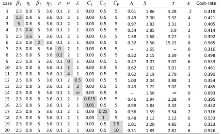
Table 2. For policy 1, optimum values of decision variables and cost-rate for various values of the model parameters. Unit cost is the cost of preventive replacement, CR. Time unit is one year.
Case 1 1 2 2 p
I
C CO CF S T K Cost-rate
[image:10.595.70.527.462.740.2](a) (b) (c)
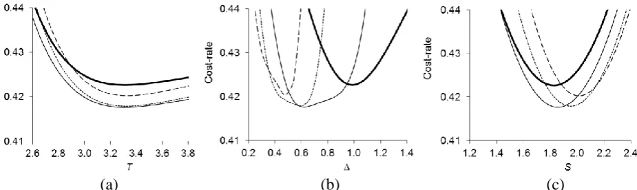
Figure 5. For policy 1, cost-rate versus (a) age at preventive replacement T, (b) interval between inspections ∆, (c) threshold age for opportunity S, for K =1 (▬▬▬), K =2 (───), K =3 (---); K=4 ( ─ ─ );other decision variables held in turn at their respective optimum values; parameter
values as case 1: 1 2.5, 1 0.8, 2 5, 2 3.6, p0.1, 2, 1, CI 0.03,
O 0.5
C , CF 5, CR 1.
Figure 5 shows that the cost-rate is most sensitive to the age limit for opportunities, S, (a 10% deviation from the optimum policy increases the cost-rate by 10% approximately) and least sensitive to T (a 10% deviation increases the cost-rate by 2.5%). This immediately indicates that utilising opportunities offers a significant cost advantage. Also, Figure 5b indicates that the inspection decision variables, K and , interact in a way that preserves the length of the inspection period, K, as we might expect.
same plant. Nonetheless, this demonstrates further the greater flexibility of this opportunistic policy over the policy without opportunity. Finally, we can see that when CO= CR (case 18) or 0
(case 9), the window of opportunity reduces to zero, as we would expect.
The mean delay time 1 / also has an important influence on the results. If the power of the observation or diagnosis of a defect becomes restricted, reflected in a decreasing mean delay time (increasing , case 12 to 1 to 13 and 14), the age threshold to enjoy an opportunity S, decreases, wherein opportunities for replacement are utilised in earlier life. Thus, opportunistic maintenance can be used to compensate for less precision in knowledge about the state of the system. In the limit (case 14), when there is no information about defects (zero delay time), the best policy is opportunistic replacement. Further, it is interesting that the influence of on K* is non-monotonic; initially K* increases with , but then for very large inspection becomes ineffective.
Finally, in relation to Table 2, we make some brief points. Comparison of cases 1-5 shows that the base case is an interesting case. Sensitivity to cost parameters is somewhat predictable: greater failure cost (case 19 to 1 to 20) leads to less inspection; cheaper inspection cost (cases 16 to 1 to 15) leads to more inspections.
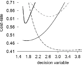
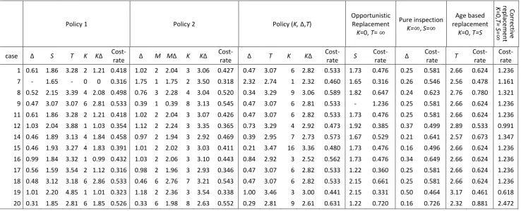
[image:12.595.207.380.534.671.2]Table 3 compares the full policy (policy 1) with a number of restricted policies, including policy 2, which itself allows for opportunities to be utilised but in a manner that is easier to manage. These comparisons are presented for some of the more interesting cases. Broadly speaking, it is the cost-rate comparisons that are most interesting here. These demonstrate the comparative economic benefits of these competing policies. Cost-rate differences in the base case are quite large (Figure 6). Here, both the pure inspection policy and the pure age based replacement policy are cost-inefficient (approximately 50% more expensive), but that an opportunistic policy is closer to the most flexible policy. Of course, this is to an extent determined by the relative cost of replacement at opportunity CO. Nonetheless, it underlines the usefulness of this policy extension. Another point is that policy 2 appears more sensitive than policy 1 to some parameter changes. An example can be seen on cases 19 and 20, where the variation in the cost of failure leads to a large change in the policy: from K 3, and M 2 in the base case to K 8 and M 6 when CF doubles.
Figure 6. Cost-rate for various special cases of policy 1: versus Δ for pure inspection policy, K=∞,
(▬▬▬);versus T for age based replacement, K=0, S=T, (▬ ● ▬); versus S for opportunistic replacement, K=0, T= ∞, (_____);versus T for policy 1with K =2 ( ─ ─ ). Other decision variables are held in turn
12
Table 3. Comparison of policies 1 and 2 and special cases: policy (K,Δ,T) (Scarf et al., 2009); opportunistic replacement (Dagpunar, 1996); pure delay time inspection (Christer, 1999), age based replacement; and corrective (failure based) replacement. Comparisons are made for some of the numbered
cases of Table 2.
Policy 1 Policy 2 Policy (K, Δ,T)
Opportunistic Replacement
K=0, T= ∞
Pure inspection
K=∞, S=∞
Age based replacement
K=0, T=S
Correc
tiv
e
re
p
lace
m
en
t
K
=0,
T=
S
=
∞
case Δ S T K KΔ
Cost-rate Δ M MΔ K KΔ
Cost-rate Δ T K KΔ
Cost-rate S
Cost-rate Δ
Cost-rate T
Cost-rate
The benefit of policy 1 over other policies can be analysed for individual parameters. Figure 7 shows the percentage cost-reduction for different values of μ (Figure 7a) and p (Figure 7b) for each policy, with other parameters at values in the base case. Figure 7a shows that as the opportunity rate increases the cost-benefit of policy 1 increases, except in comparison to the pure opportunistic replacement policy, as we would expect. The advantage over policy 2 is only slight however, indicating that this simpler policy may be the most appropriate for practice. For Figure 7b the picture is complicated. Nonetheless, it appears that while the cost-benefit of inspection increases with increasing p, the utilisation of opportunities has decreasing cost-benefit. This is likely because for large p (poor quality replacement at its most extreme) inspection becomes the dominant maintenance action. Thus utilisation of opportunities then is relatively more important provided p is not too large.
(a) (b)
Figure 7. Cost reduction (%) for policy 1 compared to policies that are special cases: (a) as a function of μ, (b) as an function of p. Policy 2 (S=MΔ, T=KΔ) (▬ ▬ ▬); opportunistic replacement
(K=0, T= ∞) (▬▬ ● ●); age based replacement (K=0, S=T) (▬▬▬); corrective maintenance (K=0, T=
∞, S=∞) (▬▬ ▬); pure inspection (K=∞) (● ● ● ●); policy (K, Δ,T) (S=T) (____) .
5 CONCLUSION
We analyse an opportunistic replacement policy that is a generalisation of a hybrid inspection and replacement policy proposed by Scarf et al. (2009). In addition to preventive replacement at the end of the wear-out phase at age T, the policy allows preventive replacement to take place opportunistically, at a cost discount, any time after age S. Such opportunities may arise as the results of stoppages, planned or unplanned, to a plant of which the system under consideration is a part. In this way, the opportunistic policy may simplify maintenance planning since such opportunities may arise with less uncertainty than scheduled age-based replacements. This is because age-based replacements do not occur periodically, unlike block replacements. The hybrid policy is a natural one where replacements are of variable quality and in the extended policy we persist with this notion of heterogeneous component lifetimes.
While notionally the system of interest is a one-component system, implicitly this is part of a large multi-component system, and it is this greater part that generates the opportunities. Thus, the policy and model we propose are applicable to and offers benefits for the maintenance of multicomponent systems.
Summarising some of the finer points of detail about the proposed policy, we find that when the cost of opportunistic replacement is small relative to the cost of preventive replacement at the end of the wear-out phase and the rate of arrival of opportunities is relatively high, preventive replacement is no longer necessary. This is not surprising. Also, when the arrival of the defects for strong components is relatively unpredictable, the best policy may also be to only await an opportunity. Furthermore, we observe that when there is little information about defects the best policy is opportunistic replacement. On the other hand, if the quality of replacements is poor then the utilisation of opportunities is relatively less important.
Finally, we note that the cost advantage of the principal policy, policy 1, over the simpler hybrid opportunistic policy, policy 2, is only small, indicating that the simpler policy may be the most appropriate for practice.
For further research, we may focus on deeper analysis of the trade-off between the theoretical effectiveness and the ease of application in practice of a maintenance policy, by investigating in particular some further strategies that make maintenance policies more applicable. Another direction to consider is the use of multi-criteria analysis for applications to service systems, where the consequences of failure go beyond the cost dimension.
ACKNOWLEDGEMENTS
The work of Cristiano Cavalcante and Rodrigo Lopes has been supported by CNPq (Brazilian Research Council).
REFERENCES
Attardi, L., Guida, M., & Pulcini, G. (2005). A mixed-Weibull regression model for the analysis of automotive warranty data. Reliability Engineering & System Safety, 87(2), 265-273.
Barlow, R. E., & Proschan, F. (1996). Mathematical Theory of Reliability. Society for Industrial and Applied Mathematics.
Berrade, M.D., Cavalcante, C.A.V., & Scarf, P.A. (2012). Maintenance scheduling of a protection system subject to imperfect inspection and replacement. European Journal of Operational Research, 218(3), 716-725.
Berrade, M.D., Scarf, P.A., & Cavalcante, C.A.V. (2017). A study of postponed replacement in a delay time model. Reliability Engineering & System Safety (in press).
https://doi.org/10.1016/j.ress.2017.04.006.
Berrade, M,D,. Scarf, P.A,, Cavalcante, C.A.V., & Dwight, R.A. (2013) Imperfect inspection and replacement of a system with a defective state: a cost and reliability analysis. Reliability Engineering and System Safety, 120(1), 80-87.
Budai, G., Dekker, R., & Nicolai, R.P. (2008) . Maintenance and production: A review of planning models. In Kobbacy K., Murthy D.N.P. (eds.) Complex System Maintenance Handbook,
Springer, pp.321-344.
Castet, J-F., & Saleh, J.H. (2010). Single versus mixture Weibull distributions for nonparametric satellite reliability. Reliability Engineering & System Safety, 95(3), 295-300.
Christer, A.H. (1987). Delay-time model of reliability of equipment subject to inspection monitoring. Journal of the Operational Research Society, 38(4), 329-334.
Christer, A.H. (1999). Developments in delay time analysis for modeling plant maintenance.
Journal of the Operational Research Society, 50(11), 1120–1137
Christer, A.H., & Wang, W. (1995). A delay-time based maintenance model for a multi-component system. IMA Journal of Management Mathematics,6(2), 205-222.
Dagpunar, J. S. (1996). A maintenance model with opportunities and interrupt replacement options.
Journal of the Operational Research Society, 47(11), 1406-1409.
De Almeida, A. T., Cavalcante, C. A. V., Alencar, M. H., Ferreira, R. J. P., de Almeida-Filho, A. T., & Garcez, T. V. (2015). Multicriteria and multiobjective models for risk, reliability and maintenance decision analysis. Springer.
Dekker, R., & Smeitink, E. (1991) Opportunity-based block replacement. European Journal of Operational Research, 53(1), 46-63.
Ding, F., & Tian, Z. (2011). Opportunistic maintenance optimization for wind turbine systems considering imperfect maintenance actions. International Journal of Reliability, Quality and Safety Engineering, 18(5), 463–481.
Gales, T. (2015) Pump reliability in the food and beverage sectors. Maintenance and Engineering,
September 2015, pp.6-10.
Garambaki, A.H.S., Thaduri, A., Seneviratne, A.M.N.D.B., & Kumar, U. (2016). Opportunistic inspection planning for railway emaintenance. IFAC-PapersOnLine, 49(28), 197-202.
Hu, J., & Zhang, L. (2014). Risk based opportunistic maintenance model for complex mechanical systems. Expert Systems with Applications, 41(6), 3105-3115.
Laggoune, R., Chateauneuf, A., & Aissani, D. (2010). Impact of few failure data on the opportunistic replacement policy for multi-component systems. Reliability Engineering & System Safety, 95(2), 108–119.
Lee, H., & Cha, J. H. (2016). New stochastic models for preventive maintenance and maintenance optimization. European Journal of Operational Research, 255(1), 80-90.
Lee, H., Cha, J. H., & Finkelstein, M. (2016). On information-based warranty policy for repairable products from heterogeneous population. European Journal of Operational Research, 253(1), 204-215.
Mohamed-Salah, A-K.D., & Ali, G. (1999). A simulation model for opportunistic maintenance strategies. In Proceedings of International Congress of Energy Technologies and Factory Automation, Vol.1, Barcelona, 703–708.
Nilsson, J., Wojciechowski, A., Strömberg, A-B., Patriksson, M., & Bertling, L. (2009). An opportunistic maintenance optimization model for shaft seals in feed-water pump systems in nuclear power plants. In 2009 IEEE Bucharest Power Tech.
Peng, H. & Zhu, Q. (2017). Approximate evaluation of average downtime under an integrated approach of opportunistic maintenance for multi-component systems. Computers & Industrial Engineering, 109, pp 335-346.
Ross, S (1996) Stochastic Processes, Wiley, New York.
Scarf, P.A. (1997). On the application of mathematical models in maintenance, European Journal of Operational Research, 99(3), 493-506.
Scarf, P.A., & Cavalcante, C.A.V. (2010). Hybrid block replacement and inspection policies for a multi-component system with heterogeneous component lives. European Journal of
Operational Research, 206(2), 384-394.
Scarf, P.A., Cavalcante, C.A.V., Dwight, R., & Gordon, P. (2009). An age based inspection and replacement policy for heterogeneous components. IEEE Transactions on Reliability, 58(4), 641–648.
Scarf, P.A., & Deara, M. (1998). On the development and application of maintenance policies for a two-component system with failure dependence, IMA Journal of Mathematics Applied in Business & Industry 9(2), 91-107.
Scarf, P.A., Dwight, R., & Al-Musrati, A. (2005). On reliability criteria and the implied cost of failure for a maintained component. Reliability Engineering and System Safety,89(2), 199-207. Shafiee, M., Finkelstein, M., & Bérenguer, C. (2015). An opportunistic condition-based
maintenance policy for offshore wind turbine blades subjected to degradation and environmental shocks. Reliability Engineering & System Safety 142, 463-471.
Tan, J.S., & Kramer, M.A. (1997). A general framework for preventive maintenance optimization in chemical process operations. Computers & Chemical Engineering, 21(12), 1451-1469. Vu, H.C., Do, P., Barros, A., & Bérenguer, C. (2015). Maintenance planning and dynamic grouping
for multi-component systems with positive and negative economic dependencies. IMA Journal of Management Mathematics, 26(2), 145-170.
Wang, W., & Christer, A.H. (2003). Solution algorithms for a nonhomogeneous multi-component inspection model. Computers & Operations Research, 30(1), 19-34.
Wang, W., Scarf, P.A., & Smith, M. (2000). On the application of a model of condition based maintenance. Journal of the Operational Research Society 51(11), 1218-1227.
Wildeman, R.E., Dekker, R., & Smit, A.C.J.M. (1997). A dynamic policy for grouping maintenance activities. European Journal of Operational Research, 99(3), 530-551.
Xia, T., Jin, X., Xi, L., & Ni, J. (2015). Production-driven opportunistic maintenance for batch production based on MAM–APB scheduling. European Journal of Operational Research, 240(3), 781-790.
Xia, T. B., Tao, X. Y., & Xi, L. F. (2017). Operation process rebuilding (OPR)-oriented maintenance policy for changeable system structures. IEEE Transactions on Automation Science and Engineering, 14(1), 139-148.
Xia, T., Xi, L., Pan, E., Fang, X., & Gebraeel, N. (2017). Lease-oriented opportunistic maintenance for multi-unit leased systems under product-service paradigm. Journal of Manufacturing Science and Engineering, 139(7), 071005.
Xia, T., Xi, L., Pan, E., & Ni, J. (2016). Reconfiguration-oriented opportunistic maintenance policy for reconfigurable manufacturing systems. Reliability Engineering & System Safety (in press). Yildirim, M., Gebraeel, N., & Sun, X. (2017). Integrated predictive analytics & optimization for
opportunistic maintenance and operations in wind farms. IEEE Transactions on Power Systems (in press).
Zhang, M., Ye, Z., & Xie, M. (2014). A condition-based maintenance strategy for heterogeneous populations. Computers & Industrial Engineering, 77, 103-114.
Zhang, X., & Zeng, J. (2017). Joint optimization of condition-based opportunistic maintenance and spare parts provisioning policy in multiunit systems. European Journal of Operational
Research, 262(2), 479-498.
Zheng, X. (1995) All opportunity-triggered replacement policy for multiple-unit systems. IEEE Transactions on Reliability, 44(4), 648-652.