Modulation Classification Algorithm for Software Radio Multiple Phase Shift Keying Signals, Using Zero Crossing Techniques

(1)

International Journal of Emerging Technology and Advanced Engineering

Website: www.ijetae.com (ISSN 2250-2459,ISO 9001:2008 Certified Journal, Volume 5, Issue 10, October 2015)

35

Modulation Classification Algorithm for Software Radio

Multiple Phase Shift Keying Signals, Using Zero Crossing

Techniques

Ishmael Zibani

1

, Edwin Matlotse

2

, Maungo S. Mmusi

3

1,2_{Department of Electrical Engineering, University of Botswana, Botswana.} 3

Botswana Power Corporation, Lobatse, Botswana.

Abstract—Software Radio is a multimode, multiband and multi standard device. So an automatic modulation scheme will be necessary to identify an unknown received signal, in the presence of noise. As the channel capacity varies, modulation scheme switching enables the baud rate to be altered in order to maximize channel capacity usage. The algorithms proposed, differ in their sensitivity to SNR, the type of modulation that they can deal with and the usable applications. In this study, we are proposing a multiple phase shift keying, MPSK modulation recognition technique based on Zero Crossing of an intercepted signal. Frequency and Phase Histograms play the role of features. More precise zero crossing points are generated using a proposed moving filter algorithm, MFA. The number of unique modulo differences between successive phases gives the value M of the MPSK signal. Our method is simple, fast, robust and efficient. Correct classification is achievable for SNR>0dB. Decision about modulation type is based on one segment, which is 1.7066ms. The design was successfully programmed into the Flex 10K0 FPGA device, housed in a ALTERA Development Board.

Keywords— Automatic Modulation, Histograms, MFA, SNR, Software Radio, Zero Crossings.

I. INTRODUCTION

Automatic modulation recognition has many important applications in communications such as signal confirmation, interference identification, monitoring, spectrum management, surveillance, identification of non-licensed transmitters, electronic warfare, threat analysis, specific emitter identification, acquiring targets, homing, control of communication quality and reconfigurable receivers. It also enables correct demodulation of a received signal without a priori modulation scheme knowledge. The most attractive application areas are automatic modulation recognition in software radio and other reconfigurable communication systems.

Adaptive modulation, where the aim is to maximize channel capacity usage by switching modulation scheme (from say, BPSK to QPSK) in order to vary the baud rate as the channel signal to noise ratio (SNR) varies, is possible once the modulation scheme in use can be identified [1 and 2].

The main goal of any identification scheme is to achieve high classification accuracy. Beside the accuracy, merits as the complexity of the implementation, the number of samples used in the proposed algorithm, and the processing overhead are important and must be considered while designing for some applications. As an example, for Software Radio implementation employing real-time modulation scheme recognition, the techniques must have a processing time overhead that still allows the software radio to maintain its real-time objectives [3].

In modern communication systems, the digital modulation techniques rather than the analogue ones are frequently used. So, the current trend is the digital modulation identifiers. Because of the classified nature of the problem, the open literature does not contain all the information on the subject of modulation identification. Until now, there are two main approaches for the modulation identification process. The first is a decision theoretic approach; the other approach is the statistical pattern recognition. Also, there are five methods of modulation identification. They are: (1) spectral processing, (2) instantaneous amplitude, phase and frequency parameters, (3) instantaneous amplitude, phase and frequency histograms, (4) combination of the previous three methods and (5) universal demodulators [4].

(2)

International Journal of Emerging Technology and Advanced Engineering

36

The hardware implementation of this identifier is excessively complex. He claimed that error-free modulation identification was achievable at SNR > 18 dB. Polydoros et al. [6] follow the decision theoretic approach to discriminate between PSK2 and PSK4 signals. Their classifier is less robust in the sense that signal parameters such as the initial phase and the symbol rate need to be available to the classifier. Huse et al. [7] follow the decision theoretic approach. Their identifier is used only for constant amplitude signals (CW, MPSK and MFSK). They claimed that successful modulation identification is valid for SNR > 15 dB. In [8], the same authors used their approach to estimate the number of levels in MPSK signals. They claimed that the eighth moment is sufficient to classify PSK2 signals with reasonable performance. Mammone et al. [9] follow the pattern recognition approach. Through simulations they demonstrate that the classifier performs well for SNR > 35 dB. Dominguez et al. [10] follow the pattern recognition approach. This classifier is a general approach for both analogue and digital modulations. However, they claimed that this recognizer performed well at SNR > 40 dB. But at SNR = 10 dB the probability of correct modulation recognition is 0% for all digital modulation types except for PSK4 (= 7%) and at 15 dB the performance is still wanting especially for FSK4 (= 56%), FSK2 (=84%) and ASK4 (= 87%). However, it should be noted that the work in [10] attempts to identify digital as well as analogue modulations. Keith et al [11] proposed a technique for a real-time software radio using general-purpose processor and is based on modified pattern recognition and signal space approaches. The technique can be used for identifying both analogue and digital modulation schemes. To increase the probability of correct classification for a short data record, Liang and Ho [12] proposed an algorithm using a two element antenna array receiver for BPSK and QPSK classification. The unknown phase shift between the two received signals due to the spatial separation of the antenna elements is estimated using maximum likelihood. They used this value to perform the generalized likelihood ratio test for classification.

This paper addresses the problem of modulation identification of MPSK signals, with specific attention to BPSK and QPSK. Polydoros et al [6] addresses the same BPSK and QPSK case using quasi Log-Likelihood ratio (qLLR) rule. Although the qLLR performed better than phased-based and square-law classifiers, the initial phase, carrier frequency and symbol rate need be known precisely.

The work presented here, closely relates to the work done by Hsue and Soliman, [7] in which they used a crossing based classifier. The authors estimated the zero-crossing variance, carrier-to-noise ratio (CNR), and carrier frequency by using these techniques. The phase deference and zero-crossing interval histograms were used as the features for recognition of the CW, MPSK, and MFSK modulated signals. The main draw back of this algorithm is the large computational overhead required and also the fact that high performance classification needs the SNR to be 15dB or above.

We propose simple algorithms based on frequency and phase parameters which are related to zero-crossings of the received signal. Our method needs fewer calculations and has a simple hardware implementation. The rest of the paper is organized as follows: Section 2 presents the proposed technique. The Moving Filter Algorithm is discussed in Section 3, while in Section 4, we show how we estimate the carrier frequency. Section 5 illustrates the MPSK algorithm itself. We conclude with Section 7. The

results are presented in Figures 4.2, 5.3, 5.4 and in section 6.

II. PROPOSED TECHNIQUES

The performance of modulation recognition schemes is degraded by the effect of white noise. Prior to modulation recognition, we reduce the effect of noise using Moving Filter Algorithm, MFA, so as to produce well defined zero crossing points. The filtering action of MFA does not alter the original signal in any way. Let the received signal be denoted by,

r(t)=d(t)+n(t) (1)

where d(t) is the modulated signal mixed with Additive White Gaussian Noise, AWGN, n(t).

The modulated signal can be modeled by,

d(t) = A*Sin{2π*fC + Φ(t)} (2)

where, A is the amplitude, fC is the carrier frequency, and Φ(t) is the phase angle of the modulated signal.

For BPSK, Φ(t) = 0, π, and for QPSK Φ(t) = 0, 2

 π, 2

3

(3)

International Journal of Emerging Technology and Advanced Engineering

37

III. MOVING FILTER ALGORITHM

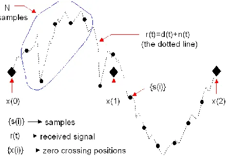
[image:3.612.57.281.262.417.2]

The original signal d(t) is contaminated with white Gaussian noise n(t) to give the received signal r(t), which is sampled to give sample sequence, {s(i)}. Suppose we choose N consecutive samples from {s(i)} (see Figure 1). The polarity of the majority of the samples will indicate whether the signal is predominantly positive or negative in that region. So for a more precise zero crossing location, we take a global decision based on N samples instead of one sample as is the conventional way.

Fig. 1 The Moving Filter Algorithm process

Let us describe the decision on the sign of r(t) based on

the N samples to be



N

s

(

i

)

_{. We can also define the}

current decision as N

s

(

i

)





and the previous decision as

)

(i

s

N 



. The decisions are based on whether r(t) is

positive (

r

(

t

)



0

), or negative (

r

(

t

)



0

). We have a zero crossing point x(i) if



(



)



N _and



(



)



N _{are different.}

We define,



N

(

s

(

i

))

_{as in equation in 3 below.}























      1 1

0 ))

(

0 ))

(

1

1 ))

(

_C _k

k i k C k i N

i

s

sign

i

s

sign

if

i

s

, (3)

where,

(

)

0

0 )

(

1

1 ))

(



















t

r

t

r

i

s

sign

,

and











search

course

N

search

fine

c

1

Note that if we are far from the natural zero crossing

point,



(



)





(



)

 

N

N _{, and we use C=N. Here, we}

perform a course search to locate the zero crossing point. There is no overlap between current samples, N+ and previous samples, N-. On the other hand, if

)

(

)

(











  N

N _{, we use C=1 for a fine search in locating} the zero crossing point. Here, we have an overlap so that, N+ and N-, differ only in one position. The zero crossing point, x(i) will be precisely defined this way.

Now we define the MFA function, Ψ acting on the received sequence {s(i)} to produce precise zero crossing sequence, {x(i)}, using sample size, N, and m being the

total number of samples. N < H, where c s f f H 2 

. The MFA function is given in equation 4 below,

, ) ( )) (

(s i x j k

N  

 , 1 1 , , )), ( ( )) ( ( )), ( ( )) ( ( , 1 ,                       

 _ _ orN

c c c k k c k k i s i s i s i s j j j N N N N N m k

while,  

_.

₍₄₎

For our simulations, we used N=10. In this case, the MFA equation becomes,

,

)

(

))

(

10

s

i



x

j



k



, 10 1 1 , , )), ( ( )) ( ( )), ( ( )) ( ( , 1 , 10 10 10 10                         _ _   or c c c k k c k k i s i s i s i s j j j 10 ,km

while _. ₍₅₎

When the condition



(



)





(



)

 

N

N _{is first detected,} we go back one iteration, and then use equation 5 with C=1. When this condition is detected for the second time, x(j) will be a zero crossing point, we increment j so that we don’t overwrite the previous x(j). When the condition

)

(

)

(











  N

(4)

International Journal of Emerging Technology and Advanced Engineering

38

The MPSK detection algorithm only uses R(i)) as given in equation 6 below. Thus,

0

0 cov

cov

0

1 )

(













vale

value

sample

ered

re

ered

re

if

i

R

(6)

IV. ESTIMATING THE CARRIER FREQUENCY The MPSK algorithm uses half the period of the carrier frequency, called H. the MFA algorithm produces more precise zero crossing positions denoted by {x(i)}. Even so, we still get invalid zero crossing points due to excessive noise or phase change. The zero crossing difference

sequence, {y(i)} is defined as

y

i



x

i



x

i1





x

i_. Conventionally, the carrier frequency, fc is estimated by





w

i i s c

y

f

w

f

1

2

1

. where w is the total number of half waves received. Invalid zero crossing points will affect the accuracy of fc. In our proposal, instead of averaging all {y(i)}, we average together y(i) which have the same values. Invalid intervals will form small groups of y(i), while valid ones form large groups of y(i). A threshold will eliminate invalid intervals, so they won’t affect the calculation of fc and hence H.

Let z = number of zero crossings received from MFA algorithm. Then we will have z–1 intervals. Assuming AWGN, the noise can only reduce the interval of a half period, not increase it. Hence the maximum length of interval yi is,

H

f

y

c s



2

max

(7)

Groups of different intervals are formed using the equation,



 



1

))

(

}

{

z

i

y

Y

y

i

Y

i

(8)

Normalization of the above equation gives,

max

^

_{

_}

}

{

_Y

Y

yi

i y

Y



(9)

[image:4.612.333.559.233.423.2]

The Block diagram of Figure 2 summarizes the process of estimating the carrier frequency. If yi is received, the decoder enables the corresponding AND gate so that Yi is incremented. YH corresponds to the carrier frequency, and theoretically will have the largest value. Figure 3 shows that indeed a normalized frequency histogram for QPSK gives a peak response at the carrier frequency of 1.5kHz. The SNR used is 7dB.

[image:4.612.320.570.444.645.2]

Fig. 2 Simple Block diagram to estimate fc.

(5)

International Journal of Emerging Technology and Advanced Engineering

39

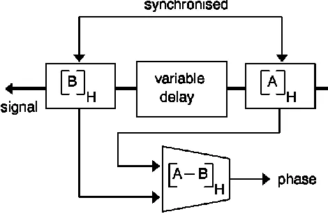
V. THE MPSKPHASE DETECTION ALGORITHM The operation of the MPSK algorithm relies on the fact that the modular difference between successive valid intervals gives phase difference, which identifies the MPSK signal. Figure 4 gives a block diagram of the MPSK phase detection circuit.

Modulo H counters, A and B are synchronised on every valid half cycle. The difference between them gives the phase angle. A half cycle is said to be valid if it contains H

samples. Likewise, a zero crossing point

x

i_{is considered}

valid if



x

i



(

x

i



x

i1

)



H





_{, where}



_{is the}

[image:5.612.101.556.98.730.2]

uncertainty in H. In between consecutive valid half cycles, there could be noise, a phase change or both. This constitutes the variable delay. If there is a symbol transmitted, the phase difference will be non-zero, otherwise zero. The number of different phase changes detected above a certain threshold, gives the value, M.

Fig. 4 MPSK Phase Detection block diagram

Because a phase change gives rise to invalid half cycles, some points, x(i) will not be valid. But we are only interested in taking the difference between valid crossings. Therefore we define another sequence, {q(x(i)}, given by

invalid

valid

i

x

i

x

i

x

q

)

(

)

(

,

0 ,

1 ))

(











. Hence the phase

change,



is given by,

H j x q j

i x q i k

x

















 1 ( ( )) 1 ))

( (



,

utive

con

j

x

q

i

x

q

for

(

)),

(

))

sec

_. ₍₁₀₎

The sign of the phase angle is given by,

1 ) (

)

lg

(

)

(log

),

(

)

(

),

(

)

(

)

(

















i q j

i

j i

k

ebra

a

ic

h

sign

h

sign

h

sign

h

sign



(11)

where, hi and hj are valid half cycles enclosing



i. The waveform of hj is extended so that sign( i



) is taken at a point j where q(i)=1.

Figure 5 shows a logic diagram for the MPSK detection. Both A and B are modulo H counters. B is reset on every zero crossing while A is reset on every valid zero crossing.

If

 

B

H_{=0 when x}_i_{is received, then x}_i_{is a valid zero} crossing point. Then the contents of

 

A

H_{are loaded into}

the latch before

 

A

H_{is reset. The output of the latch} becomes the phase.

Fig. 5 MPSK detection logic diagram

[image:5.612.50.285.358.516.2]

(6)

International Journal of Emerging Technology and Advanced Engineering

40

[image:6.612.326.557.130.320.2]

The number of peaks (above a suitable threshold) in a phase histogram corresponds to the value M, of an MPSK signal. For example, 2 peaks will give BPSK (Figure 6), 8 peaks will give 8PSK, etc.

[image:6.612.47.291.182.571.2]

Fig. 6 BPSK phase histogram.

Figure 7: QPSK phase histogram

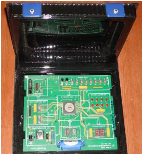
VI. IMPLEMENTATION OF PROPOSED DESIGNS ON FPGA Figure 8 shows the design of the MPSK logic diagram of figure 5 using ALTERA’s Max Plus design environment. The carrier frequency of figure 2 was designed the same way. After designing all the project components, the whole project was implemented on a 10K20 programmable FPGA logic device, within ALTERA’s Development Board (figure 9).

Fig. 8. MPSK logic design using ALTERA design environment.

Figure 9. ALTERA MAX PLUS Development Board.

VII. CONCLUSIONS

[image:6.612.328.558.346.596.2]

(7)

International Journal of Emerging Technology and Advanced Engineering

41

Memory requirements are very low as the samples are discarded after identification of a symbol. The action of MFA algorithm greatly enhances symbol identification. Parameters like carrier frequency, symbol timing, etc, which usually are a necessity with other modulation recognition algorithms, are not required here. Since each symbol is uniquely identified, no demodulation process is necessary thereafter. Preferred method of implementation is using FPGAs as they are fast, consumes less power and are reusable.

REFERENCES

[1] E. E. Azzouz and A. K. Nandi. Automatic Modulation Recognition of Communication Signals. Publisher: Kluwer Academic Publishers, 1996.

[2] Dillinger M., Madani K. and Alonistioti N., In: Software Defined Radio, Architectures, Systems and Functions. Editors: John Wiley & Sons Ltd. Publishing, U.K., John Wiley & Sons Ltd. pp. 47-72, 2003.

[3] Ferdinand Liedtke. Adaptive procedure for automatic modulation recognition. Journal of telecommunicatuions and information technology, April 2004.

[4] Octavia A. Dobre1, Ali Abdi2, Yeheskel Bar-Ness2 and Wei Su3. A Survey of Automatic Modulation Classification Techniques: Classical Approaches and New Trends. Sarnoff Symposium, Princeton, NJ, USA.

[5] F. Liedtke. Computer Simulation of an automatic classification procedure for digitally modulated communications signals with unknown parameters. Signal Processing, Volume6, No. 4, pp.311-323, March 1984.

[6] K. Kim and A. Polydoros. Digital modulation classification: the BPSK versus QPSK case. in Proc. IEEE Conf., 1988, pp. 431-436. [7] S.Z. Hsue and Samir S. Soliman. Automatic modulation

classification using zero crossing. IEE Proceedings-F, RADAR AND SIGNAL PROCESSING, volume. 137, part F, Number 6, December 1990.

[8] Z.S. Huse and S.S. Soliman, ―Signal classification using statistical moments. 1EEE Transaction. Communications,Vol. 40, No. 5, May 1992, pp. 908-916.

[9] R.J. Mammone et al. Estimation of carrier frequency, modulation type and bit rate of an unknown modulated signal. Proc. ICC, 1987. [10] L. Vergara Dominguez, J.M. Phz Borrallo, J. Portilla Garcia and B.

Ruiz Mezcua. A general approach to the automatic classification of radiocommunication signals. Signal Processing, Vol. 22, No. 3, March 1991, pp. 239-250.

[11] Keith E. Nolan, Linda Doyle, Donald O’Mahony, Philip Mackenzie. Signal Space based Adaptive Modulation for Software Radio. WCNC 2002 – IEEE Wireless Communications and Networking Conference, Vol.3, no. 1, March 2002, pp. 435 – 440.