Neural network based colonoscopic diagnosis using on line learning and differential evolution

BIROn - Birkbeck Institutional Research Online

Magoulas, George D. and Plagianakos, V.P. and Vrahatis, M.N. (2004) Neural

network-based colonoscopic diagnosis using on-line learning and differential

evolution. Applied Soft Computing 4 (4), pp. 369-379. ISSN 1568-4946.

Downloaded from:

Usage Guidelines:

Please refer to usage guidelines at or alternatively

Birkbeck ePrints: an open access repository of the

research output of Birkbeck College

http://eprints.bbk.ac.uk

Magoulas, George D.; Plagianakos, Vassilis P. and

Vrahatis, Michael N.

(2004).

Neural network-based

colonoscopic diagnosis using on-line learning and

differential evolution.

Applied Soft Computing

4 (4)

369-379.

This is an author-produced version of a paper published in

Applied Soft

Computing

(ISSN

1568-4946). This version has been peer-reviewed but does

not include the final publisher proof corrections, published layout or

pagination.

All articles available through Birkbeck ePrints are protected by intellectual

property law, including copyright law. Any use made of the contents should

comply with the relevant law.

Citation for this version:

Magoulas, George D.; Plagianakos, Vassilis P. and Vrahatis, Michael N.

(2004).

Neural network-based colonoscopic diagnosis using on-line learning

and differential evolution.

London: Birkbeck ePrints.

Available at:

http://eprints.bbk.ac.uk/archive/00000350

Citation for the publisher’s version:

Magoulas, George D.; Plagianakos, Vassilis P. and Vrahatis, Michael N.

(2004).

Neural network-based colonoscopic diagnosis using on-line learning

and differential evolution.

Applied Soft Computing

4 (4) 369-379.

http://eprints.bbk.ac.uk

Neural Network-based Colonoscopic Diagnosis Using On-line

Learning and Differential Evolution

George D. Magoulas, Vassilis P. Plagianakos

*

and Michael N. Vrahatis

*

Department of Information Systems and Computing, Brunel University,

Uxbridge UB8 3PH, United Kingdom

Phone: +44-1895-274000, Fax: +44-1895-251686

email:[email protected]

*

Department of Mathematics and University of Patras Artificial Intelligence Research Center

(UPAIRC), University of Patras, GR-26110 Patras, Greece

Phone: +30-61-997374, Fax: ++30 61 992965

email:{vpp,vrahatis}@math.upatras.gr

ABSTRACT: In this paper, on-line training of neural networks is investigated in the context of

computer-assisted colonoscopic diagnosis. A memory-based adaptation of the learning rate for the on-line

Backpropagation is proposed and used to seed an on-line evolution process that applies a Differential

Evolution Strategy to (re-)adapt the neural network to modified environmental conditions. Our approach

looks at on-line training from the perspective of tracking the changing location of an approximate solution of

a pattern-based, and, thus, dynamically changing, error function. The proposed hybrid strategy is compared

with other standard training methods that have traditionally been used for training neural networks off-line.

Results in interpreting colonoscopy images and frames of video sequences are promising and suggest that

networks trained with this strategy detect malignant regions of interest with accuracy.

KEYWORDS: Minimally invasive imaging procedures, Backpropagation networks, Medical image

interpretation, On-line learning, Differential evolution strategies, Artificial evolution.

1. INTRODUCTION

In medical practice, endoscopic diagnosis and other minimally invasive imaging procedures, such as computed

tomography, ultrasonography, confocal microscopy, computed radiography, or magnetic resonance imaging,

are now permitting visualization of previously inaccessible regions of the body. Their objective is to increase

the expert’s ability in identifying malignant regions and decrease the need for intervention while maintaining

the ability for accurate diagnosis. Furthermore, it may be possible to examine a larger area, studying living

tissue in vivo - possibly at a distance [5] - and, thus, minimise the shortcomings of biopsies, such as limited

In this paper, we focus on neural network-assisted diagnosis of colonoscopy images. Colonoscopy is a

minimally invasive technique for the production of images of the colon: a narrow pipe like structure, an

endoscope, is passed into the patient’s body. Video endoscopes have small cameras in their tips, when passed

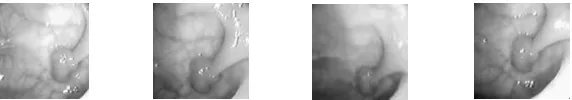
into a body, what the camera observes is displayed on a television monitor (see Figure 1 for frame samples

of a video sequence). The physician controls the endoscope’s direction using wheels and buttons and the

whole procedure is carried out under variable perceptual conditions (shadings, shadows, lighting condition

[image:4.595.157.443.198.248.2]

variations, reflections etc.).

Figure 1. Frames of a video sequence showing a polypoid tumor of the colon.

Neural network-based methodologies present some interesting qualities, such as learning from experience,

generalisation, and are able to handle uncertainty and ambiguity in distorted or noisy images to some extent.

Thus, these methods provide human experts with significant assistance in medical diagnosis [8], [10], [12],

[13], [23].

The use of neural networks for the detection of malignant regions in colonoscopy video sequences

encounters several problems: the time varying nature of the process; changes in the perceptual direction of

the physician; variations in the diffused light conditions. In most of these cases, off line learning or

knowledge -based approaches are not able to represent all possible variations of the environment. On-line

training and retraining allow the network to update its weights during operation by taking into account both

the already stored knowledge and the knowledge extracted from the current data, and are proposed as

alternatives to batch learning-based approaches. Of course, the main challenge when dealing with adaptive

techniques for learning, such as on-line training and retraining, is to balance the information related to

recently acquired data with the information already embodied in the network [3], [6], [27].

Thus, in this paper we explore on-line training and retraining of neural networks with the aim to detect

malignant regions in colonoscopy images though a formulation of the problem that is based on the idea of

tracking the moving “optimum” of a dynamically changing pattern-based error measure. This approach

coincides with the way adaptation on the evolutionary time scale is considered [29], and allows us to explore

and expand further research on the tracking performance of evolution strategies and genetic algorithms [2],

[29], [35]. Hence, the reader should keep in mind that in this paper we do not seek global minimisers of the

error function, but we are interested in developing an on-line evolution strategy that will converge to an

approximation of the optimum solution (the interesting topic of finding global minimisers in neural networks

The paper is organised as follows. Section 2 explains how textural variations of the tissue are modelled in

our approach. Section 3 discusses existing learning approaches, while Section 4 describes the proposed

on-line evolution strategy. In Section 5 experimental results are presented and findings are discussed. Lastly,

conclusions are drawn in Section 6.

2. TISSUE CLASSIFICATION FOR ENDOSCOPIC DIAGNOSIS

In endoscopic diagnosis, the medical expert, based on a distributed percept of local changes, interprets the

physical surface properties of the tissue - such as roughness or smoothness, regularity, and shape - to detect

abnormalities. It is important to note, however, the vast difficulties in physical attributes of the organs. For

example, in colonoscopy, no two colons are alike. Even within the same colon, one section may have very

different characteristics from another. Adjacent regions of the colon lining showing different properties are

distinguished on the basis of the textural variations of their tissue (pit patterns) [22]. These difficulties

introduce severe limitations in the use of computer-assisted endoscopic diagnosis [13], [23]. Given a medical

image, the “true” features associated with the physical surface properties of the tissue are not exactly known

to the image-interpretation system developer. Usually, one or more feature-extraction models [16], [17] are

used to provide values for each feature’s parameters. The findings are then used to infer the correct

interpretation. On this same task of interpretation on the basis of local changes of the properties of the tissue

under examination, the performance of human perception is considered outstanding. Furthermore, medical

experts have the ability to either add or remove components from an image to give meaning to what they see.

Medical experts can also adapt to changes to the extent that even a distorted image can be recognized.

In computerised systems, the classification of image regions is usually quite sophisticated and involves

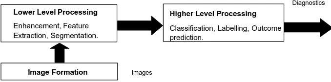
multiple levels of processing. In general, a model with three stages is employed as shown in Figure 2

(adapted from [16]).

Image Formation Images Lower Level Processing

Enhancement, Feature Extraction, Segmentation.

Higher Level Processing

Classification, Labelling, Outcome prediction.

[image:5.595.128.467.529.613.2]

Diagnostics

Figure 2. Model for diagnostic system that uses medical images.

The lower-level processing takes image pixels as input and performs various tasks such as image

enhancement, feature extraction and image segmentation. The higher-level processing takes the output from

in the higher-level processing include classification of features, detection of specific lesions and diagnosis

for various abnormalities.

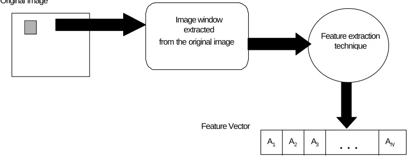
Original Image

Image window extracted

from the original image Feature extraction _technique

A1 A2 A3 AN

Feature Vector

[image:6.595.88.508.112.275.2]

. . .

Figure 3. Stages in feature extraction.

An important stage of the implementation is the feature extraction process (see Figure 3). In our experiments

the method of cooccurrence matrices was used for feature extraction. Cooccurrence matrices, [9], represent

the spatial distribution and the dependence of the grey levels within a local area. Each p(i,j) entry of the

matrices, represents the probability of going from one pixel with a grey level (i) to another with a grey level

(j) under a predefined distance and angle. From these matrices several sets of statistical measures, or feature

vectors, are computed to build different texture models. In our implementation, the colonoscopy image was

separated into windows of size 16×16 pixels with 8 pixels overlap. Then the cooccurrence matrices algorithm was used to gather information from the pixels of an image window. Four angles, namely 0?, 45?,

90?, 135?, were considered as well as a predefined distance of one pixel in the formation of the cooccurrence

matrices. Therefore, four cooccurrence matrices using the following four statistical measures were formed

(see [12] for details):

Energy-Angular Second Moment: _f

1 =

∑∑

( )

i j

j i

p , 2, ₍₁₎

Correlation:

f2 =

( ) ( )

y x g

N

i g N

j

y x

j i p j i

σ σ

µ µ

∑∑

_{= =} ∗ −

1 1

,

, (2)

Inverse Difference Moment:

f3 =

(

) ( )

pi j j

i

i j

, 1

1

∑∑

_{+ −} , (3)

Entropy:

f4 =

p

i

j

(

p

( )

i

j

)

i j

,

log

,

∑∑

 

−

, (4)

where Ng is the number of grey levels, µx, µyare the marginal mean values of x (along the horizontal pixel

deviations. Thus, a set of 16 features describing spatial distribution in each window is obtained and used to

formulate inputs for high level processing.

3. BATCH LEARNING OF MULTILAYER PERCEPTRONS

The most popular neural network model is the so-called Multi-Layer Perceptron (MLP). In an MLP, whose l

-th layer contains

N

l nodes, (l = 1,...,M), artificial neurons operate according to the following equations:

∑

− = − − = 1 1 1 , 1 l N i l i l l ij l

j w y

net (5)

)

( l

j l

j f net

y = ₍₆₎

where net_jl

is, for the j-th neuron in the l-th layer ( j = 1,...,

N

l), the sum of its weighted inputs. The weights

for connections from the i-th neuron at the (l-1) layer to the j-th neuron at the l-th layer are denoted by w_ijl−1 ,l ;

l j

y is the output of the j-th neuron that belongs to the l-th layer, and the logistic function

f netj net

l

j l

( ) (= +1 (− ))−1

exp is the j-th's neuron non-linear activation function.

Training an MLP to recognise abnormalities in image regions is typically realised by adopting an error

correction strategy that adjusts the network weights through minimisation of learning error:

∑ ∑

= =

−

=

P

p M N

j jp

M p j

t

y

E

_{1 1} 2

, ,

)

(

2

1

=

∑

= P p1

E

p

2

1

(7)

where (yj p t ) M

j p

, − , 2

is the squared difference between the actual output value at the j-th output layer neuron,

for an input sample p, and the target output value; p is an index over input-output patterns.

A variety of approaches adapted from the theory of unconstrained optimisation have been applied to the

minimisation of function E. For example, let us consider the class of batch learning algorithms that adjust the

weights according to the iterative scheme:

K , 2 , 1 , 0

1 = + =

+ _{w k}

wk k ηϕk ₍₈₎

Note that in (8) the weights of the MLP are expressed in a simplified form using vector notation. Thus, wk

defines the current weight vector, ϕk is a correction term, and

η

is the learning rate at the kth iteration.

Various choices of the correction term ϕk give rise to distinct batch learning algorithms, which are usually

classified as first-order or second-order algorithms depending on the derivative-related information they use

to generate the correction term. Thus, first-order algorithms are based on the first derivative of the learning

error with respect to the weights, while second-order algorithms on the second derivative (see [4] for a

A broad class of batch-type first-order algorithms, which are considered much simpler to implement than

second-order methods, uses the correction term ϕk =−∇E(wk). The term ∇E(wk) defines the gradient

vector of the MLP and is obtained by means of back-propagation of the error through the layers of the

network. The most popular algorithm of this class, called batch Back-Propagation (BP) applies the steepest

descent method with a constant, heuristically chosen, learning rate η that usually takes values in the interval

(0,1) [17]. Values in this interval are considered small enough to ensure the convergence of the BP training

algorithm and consequently the success of learning [4]. However, it is well known that this practice tends to

be inefficient [4], [17] and the use of adaptive learning rate strategies is suggested in order to accelerate the

learning process (see [4] and [19] for reviews on adaptive learning rate algorithms).

With regards to second-order training algorithms, nonlinear conjugate gradient methods, such as the

Fletcher-Reeves or the Polak-Ribiere methods [21], or variable metric methods, such as the

Broyden-Fletcher-Goldfarb-Shanno method [4], or even modification of Newton's method [7], [18] have been

proposed in the literature. These methods exploit derivative calculations and subminimization procedures

(e.g. the nonlinear conjugate gradient methods) and/or approximations of various matrices (e.g. the Hessian

matrix for the variable metric or quasi-Newton methods) to accelerate the learning process.

4. ON-LINE EVOLUTION STRATEGY

On-line training in neural networks is related to updating the network parameters after the presentation of

each training example, which may be sampled with or without repetition. On-line training may be the

appropriate choice for learning a task either because of the very large (or even redundant) training set, or

because of the slowly time-varying nature of the task. Although batch training seems faster for small-size

training sets and networks, on-line training is probably more efficient for large training sets and networks. It

helps to escape local minima and provides a more natural approach to learning in non-stationary

environments. On-line methods seem to be more robust than batch methods as errors, omissions or redundant

data in the training set can be corrected or ejected during the training phase. Additionally, training data can

often be generated easily and in great quantities when the system is in operation, whereas they are usually

scarce and precious before. Lastly, on-line training is necessary in order to learn and track time varying

functions and continuously (re-)adapt in a changing environment.

Despite the abundance of methods for learning from examples, there are only few that can be used

effectively for on-line learning. For example, the classic batch training algorithms cannot straightforwardly

handle nonstationary data. Even when some of them are used in on-line training there exists the problem of

“catastrophic interference”, in which training on new examples interferes excessively with previously

BP-seeded Differential Evolution (DE) strategy for on-line neural network training. Firstly, we briefly present

the on-line BP learning stage of the proposed strategy. Then we proceed by describing the on-line DE stage.

Note that the description below focuses on the problem of adapting the weights line, assuming that

on-line evolution is always activated, and does not require the input and desired output data to be known a

priori. Our experiments, reported in the next section, were also conducted under the same assumptions to test

the robustness of our approach. Note, however, that in practice, whenever the changes of the environment are

not considered significant and the performance is satisfactory, the weights and structure of the network

should remain constant [6].

4.1 ON-LINE BACKPROPAGATION LEARNING

On-line BP learning strategies are usually based on the use of stochastic gradient descent due to the inherent

efficiency of this method in time-varying environments [1], [30], [31], [33], [34]. On-line learning has been

analysed within the framework of statistics and it has been shown that it is asymptotically as effective as

batch (also called off-line) learning. However, sensitivity to learning parameters is a common drawback of

these schemes [28]. Advanced optimisation methods, such as conjugate gradient, variable metric, simulated

annealing etc., cannot be used in this context, as they rely on a fixed error surface and need information from

the whole training set [28].

In [20], a variant of the on-line BP has been proposed. The method can be considered as a meta-learning

algorithm in the sense that it learns the learning rate parameters of an underlying base learning system (i.e. of

the stochastic gradient descent). To this end, the new variant uses a memory-based learning rate adaptation

schedule that exploits gradient related information from the current as well as the two previous pattern

presentations: ) ( ), ( ) ( ), ( 1 1 2 2 2 1 1 1 1 − − − − − −

+ _{= + ∇ ∇ + ∇ ∇} k

p k p k p k p k k w E w E w E w E γ γ η

η . (9)

At the start of the learning procedure, k=0, the learning rate is set to a small positive value; e.g. the initial

learning rate was set to 0.001 in our experiments. Then, the weights are updated on-line, for each pattern p,

following the iterative scheme:

) ( 1 k p k k k w E w

w + = −η ∇ . (10)

In (9), .,. stands for the usual inner product in

R

n, E_pis the pattern-based error measure and ∇Epis the

corresponding gradient vector; η is the learning rate, and γ1, γ2are the meta-learning rates (γ1<γ2 <1).

Meta-learning rates are also in use by other on-line learning schemes, such as in [1], [30],[31],[33], and can

take various forms depending on the method. Previous experiments with the new variant have shown that the

helps the stochastic gradient descent to exhibit fast convergence and high success rate [20]. In addition, the

method is characterised by low storage requirements and inexpensive computations, as it only uses already

calculated information from the current, as well as the previous iteration. The idea of considering the

gradient of the previous iterations in a learning rate adaptation scheme has also been proposed in the context

of off-line learning. Particularly, Jacobs in the delta-bar-delta algorithm, [11], measures the running average

of the current,∇E(wk), and past partial derivatives in order to check whether the current gradient has the

same sign as the average gradient. Then the algorithm either increases the learning rate by adding a positive

constant to the current value, or decreases it by multiplying the current value with a positive, smaller than

one, constant. Finally, the weights are updated using a variant of Eq. (8), as the delta-bar-delta algorithm

needs information from the whole training set (i.e. it performs batch learning).

The on-line iterative scheme of (9)-(10) was shown to provide increased speed and higher possibility of good

performance in different classes of problems when compared against the classic on-line BP and other

meta-learning rate algorithms (see [20], [25] for details and comparisons). The role of on-line BP in the context of

computer-assisted colonoscopic diagnosis is to initialise the population of the DE strategy with an initial

approximation of the solution, as will be described below.

4.2 DIFFERENTIAL EVOLUTION STRATEGY

Evolution Strategies (ESs) are adaptive stochastic search methods that mimic the metaphor of natural

biological evolution. The main differences between ESs and Genetic Algorithms lie in that the

self-adaptation of the mutation operator is a key feature of the ESs, and in that GAs prefer smaller mutation

probability (rate) [2], [29]. Here we use the Differential Evolution strategies, which have been designed as

stochastic parallel direct search methods that can handle non-differentiable, non-linear and multimodal

objective functions efficiently, and require few easily chosen control parameters [32]. Experimental results

have shown that DE strategies have good convergence properties and outperform other evolutionary

algorithms and annealing methods [32]. To apply DE strategies to neural network training we start with a

specific number (NP) of n-dimensional weight vectors, as initial population, and evolve them over time; NP

is fixed throughout the training process and the weight population is initialised by perturbing the

approximate solution provided by the on-line BP (see Relations (9)-(10)). Thus, the on-line BP seeds the DE,

so the initial population might be generated by adding normally distributed random deviations to the nominal

solution.

Let us now describe the proposed version of DE strategy that is used in the on-line evolution strategy. The

weight vectors evolve randomly with each pattern presentation (iteration) through the relation

(

r r

)

i NP

k i k best k

i k

i w w w w w

v 1 2 , 1,K

1

=

− + − + =

+ _µ

where k best

w is the best population member of the previous iteration, µ >0 is a real parameter (mutation

constant) which regulates the contribution of the difference between weight vectors, and wr₁

,

wr₂are weight

vectors randomly chosen from the population with r1,r2∈

{

1,2,K,i−1,i+1,K,NP

}

, i.e. r1,r2are random

integers mutually different from the running index i. Aiming at increasing the diversity of the weight vectors

further, a crossover-type operation is introduced in Relation (12). Thus, the so-called trial vector,

NP i

uk

i , 1,K

1 =

+

, is generated.

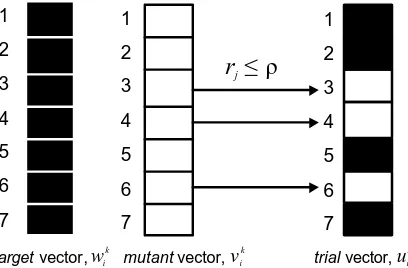
   ≠ > = ≤ = + + i j k j i i j k j i k j i rand j r w rand j r r v u and if o if , 1 , 1 , ρ ρ

. ₍₁₂₎

This operation works as follows: the mutant weight vectors, vk i NP

i , 1,K

1 =

+ _{, are mixed with the “target”}

vectors, k i

w . Specifically, we randomly choose a real number r in the interval [0,1] for each component j,

j=1,2,…, n, of k+1

i

v . This number is compared with ρ∈[0,1] (crossover constant), and if r≤ρ then the j-th

component of the trial vector uik+1 gets the value of the j-th component of the mutant vector,

1

+

k i

v ; otherwise,

it gets the value of the j-th component of the target vector, k i

w . In (12), randi is a randomly selected index

that is used to ensure the trial vector has at least one component from the mutant vector. An application

example of this operation is shown in Figure 4 for a seven-dimensional weight vector.

1 2 3 4 5 6 7 1 2 3 4 5 6 7 1 2 3 4 5 6 7

targetvector, wik mutantvector, trialvector,

[image:11.595.197.401.413.547.2]

k i v k i u

ρ

≤

j

r

Figure 4. Illustration of the crossover operation.

The trial vector is accepted for the next iteration if and only if it reduces the value of the pattern-based error

measure Ep; otherwise the old value, k i

w , is retained. This last operation, called selection, ensures that the

fitness starts steadily decreasing at some iteration, and is described in Relation (13).

The combined action of mutation and crossover operation is responsible for much of the effectiveness of DE

search, and allows DE strategies to act as parallel, noise-tolerant hill-climbing algorithms, which efficiently

search the whole space for solutions [32].

5. EXPERIMENTS AND RESULTS

In our experiments, the colonoscopy images and video frames were separated into windows of size 16×16 pixels with overlap of 8 pixels. Then the co-occurrence matrices algorithm was applied to gather information

regarding pixel neighbourhoods of randomly selected image windows, as described in Section 2. The

procedure results in 16-dimensional feature vectors, which are very noisy as no pre-filtering or segmentation

techniques is applied, and are used in the experiments described below. The learning parameters of the

on-line evolution strategy have been set following the recommendations of [25] and [32]: γ₁ =0.05, γ₂ =0.95,

5 . 0

=

µ , ρ=0.9. Lastly, NP=100.

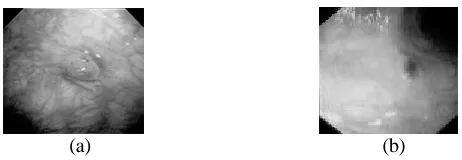
[image:12.595.179.410.346.426.2]

(a) (b)

Figure 5. Colonoscopy images used in the experiments.

In the first set of experiments, 1000 MLPs with varying number of hidden nodes (from 8 to 21) were trained

using two batch learning algorithms, the Adaptive learning rate Backpropagation (ABP) proposed by Vogl

[36], and the Levenberg-Marquardt (LM) method [7], as typical examples of first- and second- order training

algorithms respectively. The MLPs were trained using 10 normal/10 abnormal samples from image windows

that were randomly extracted from images (a) and (b) (see Figure 5) and tested with different tissue samples

taken from the two images. Note that the malignant regions in these images belong to two different types:

Image (a) is a low grade cancer, while Image (b) is a moderately differentiated carcinoma [15]. The

performance of the trained MLPs has been tested on a set of 80 texture samples (40 normal and 40

malignant) randomly selected from the two images and different from the training set. Only a small sample

out of 1000 trained MLPs of the different architectures exhibited classification success of 90% or higher.

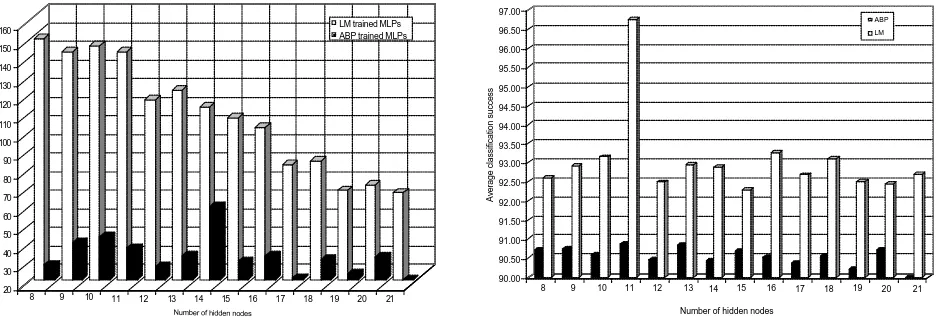
Detailed results are shown in Figure 6. More specifically, only 150 MLPs with 8 hidden nodes, out of the

1000 trained, exhibited the desired classification success (see Figure 6, left part). Note also the significant

difference in the number of the MLPs with acceptable classification success among the ABP and the LM

on the right part of Figure 6. In fact MLPs with 11 hidden nodes exhibit the highest average in classification

success (96.75%). Thus, 11 hidden node MLPs were used in the second set of experiments.

20 30 40 50 60 70 80 90 100 110 120 130 140 150 160

Number of MLPs out of 1000

1 2 3 4 5 6 7 8 9 10 11 1 2 13 14

Number of hidden nodes

LM trained MLPs ABP trained MLPs

9 11

8 10 12 13 14 15 16 17 18 19 20 21

90.00 90.50 91.00 91.50 92.00 92.50 93.00 93.50 94.00 94.50 95.00 95.50 96.00 96.50 97.00

Average classification success

1 2 3 4 5 6 7 8 9 10 11 12 13 14

Number of hidden nodes

ABP LM

[image:13.595.68.536.108.268.2]

8 9 10 11 12 13 14 15 16 17 18 19 20 21

Figure 6. Number of MLPs (out of 1000) with classification success greater than 89% (left), and average classification

success (right) for these MLPs. Results are for the images of Figure 5.

In the second set of experiments, 1000 MLPs of 16-11-2 architecture were trained off-line to detect

malignant regions in a frame of colonoscopy video sequence using a training set of 150 normal/150

abnormal patterns. Three batch-learning methods were comparatively evaluated in this round of experiments:

the Levenberg-Marquardt that exhibited good performance in the previous round, the Scaled Conjugate

Gradient (SCG) method, [21], that is considered according to the literature as a good alternative to the use of

second-order methods [17], and the Rprop algorithm, [25], which is a first-order method that applies

heuristics to adapt a different learning rate for each weight of the network and combines successfully

effectiveness with low computational requirements [17]. The percentage of classification success in testing

(test set included 3969 patterns, i.e. the whole region covered in the video frame) for the 1000 trained

networks is shown in Figure 7. One can observe that it is not easy to locate weights that will allow the

networks to detect malign ant regions with a success of over 90%. For example, in Figure 7, only 2 networks

out of the 1000 trained with the Rprop algorithm achieved recognition success from 90% to 100%. For the

SCG method the corresponding number is 3 out of 1000, while for the LM method this number is slightly

higher, as 6 out of the 1000 networks exhibited classification success between 90% and 100%. The best

result for each training method is: 92% for the Rprop, 92.4% for the LM and 92.6% for the SCG. Rprop

needs on average more epochs to converge than the SCG and LM methods but does not require heavy matrix

computations or subminimisations. As a consequence, it was observed that the average time for training with

Rprop was shorter than the corresponding time of SCG or LM. Thus, we decided to keep Rprop and run

experiments with data from other video frames of the same video sequence. The best results are summarised

0 100 200 300 400 500 600 700

Number of trained networks

50-59 60-69 70-79 80-89 90-100

Percentage of classification succes in testing

Rprop

L-M

SCG

Figure7. Generalisation results for three batch-training algorithms.

From the results of Table 1, it is clear that Rprop exhibits the best overall performance compared with ABP.

Note that the results of Tables 1 have been achieved by training off-line frame-dedicated MLPs with 11

hidden nodes using 300 patterns randomly chosen from each frame and testing using data of the same frame.

Method Frame 1 Frame 2 Frame 3 Frame 4

Rprop 92% 91% 92% 93%

[image:14.595.159.453.59.237.2]

ABP 81% 85% 83% 81%

Table 1. Best classification success for two first order batch-learning methods.

In the third set of experiments, the Rprop algorithm was compared with the classic on-line BP using data

from another frame of the same video sequence. 300 patterns were used for training and 3969 for testing (i.e.

the whole tissue region covered in the frame). The capability of the trained network (16-11-2 MLPs were

used) with the best performance in assigning appropriate characterisations (normal/abnormal) to frame

regions is shown in Table 2.

Method Abnormal (%) Normal (%) Mean (%)

Rprop 83 96 93

On-line BP 73 93 88

Table 2. Best performance in terms of generalisation for Rprop and on-line BP.

The Rprop reveals, in general, a higher percentage of success than the on-line BP. The reader should, of

course, keep in mind that Rprop minimises a batch error measure, i.e. it uses the true gradient of the error

function as it exploits information from all the training patterns. The on-line BP, on the other hand,

minimises a pattern-based error measure and works with an instantaneous approximation of the true gradient

[image:14.595.139.454.375.413.2]

(re-)adapting to modified environment conditions, while Rprop requires all information about input-output

patterns to be known a priori and, thus, fails to work when all the relevant features of the environment are

not explicitly defined in advance. However, the results of the experiments made clear that the classic on-line

BP needs further improvement in order to train networks to detect malignant regions with accuracy

comparable to batch training methods.

In the fourth set of experiments, 16-11-2 MLPs have been trained on-line to detect malignant regions in a set

of four frames from the same video sequence. The frames used in the two previous experiments were

included in the set. The networks have been trained on-line, following the iterative scheme (9) for adapting

the learning rate, to recognise patterns from the first frame. Then on-line learning with differential evolution

occurred as data from the second frame appeared at the input. The on-line evolution learning strategy

continuously adapts the network as patterns from other frames are presented in random order at the input. In

total, 1200 patterns from the four frames of the video sequence were presented to the network during the

training phase. The network was then tested using 15876 patterns from the four frames (4000 patterns

approximately cover the whole tissue region of a frame and include normal as well as malignant areas). The

average capability of the trained networks in assigning appropriate characterisations to explored colon lining

regions is presented in Table 3.

Method Frame 1 Frame 2 Frame 3 Frame 4

On-line BP 83% 84% 77% 88%

On-line BP seeded DE 93% 92% 84% 90%

Table 3. Normal/abnormal detection accuracy.

The on-line BP seeded DE scheme provides generalisation results close to the best results obtained by the batch training

methods, as reported in the previous experiments. For example, the best SCG-trained dedicated network in the second

experiment (trained off-line and tested using data from Frame 1) had 92.6% success, and the best Rprop-trained

dedicated network in the third experiment (trained off-line and tested using data from Frame 2) had 93% success.

6. CONCLUSIONS AND FUTURE WORK

In this paper a new scheme for neural network-based colonoscopic diagnosis was introduced. The proposed

on-line evolution strategy can be considered as a hybrid algorithm. It uses an on-line Backpropagation

strategy with adaptive learning rate to seed the initial population of the on-line Differential Evolution

strategy. In our experiments, neural networks trained with the proposed on-line evolution strategy exhibited

satisfactory performance under changing environmental conditions, as data from different frames were

In the reported experiments no emphasis was put in fine-tuning the heuristic parameters of our scheme;

classic values found in the relevant literature of Differential Evolution strategy were used instead. In future

work we will fully investigate the properties, study the effect of the heuristic parameters and evaluate the full

potential of the hybrid learning strategy in colonoscopic diagnosis by means of extensive testing on long

video sequences and interpretation of complex tissue regions.

ACKNOWLEDGEMENTS

The authors gratefully acknowledge the contribution of Dr. S. Karkanis (Technological Educational Institute

of Lamia, Greece) and D. Iakovidis (University of Athens, Greece) in the acquisition of video sequences and

extraction of features.

REFERENCES

[1] Almeida, L.B., Langlois, T., Amaral, J.D., and Plankhov, A. (1998). “Parameter adaptation in stochastic optimisation”, in “On-line Learning in Neural Networks”, Saad, D. (ed.), 111-134, Cambridge University Press.

[2] Angeline, P. (1997). “Tracking extrema in dynamic environments”', 6th Annual Conference on Evolutionary Programming VI, 335-345, Springer.

[3] Anguita D. (2001). “Smart adaptive systems: state of the art and future directions of research”, in Proceedings of the European Symposium on Intelligent Technologies, Hybrid Systems and their Implementation on Smart Adaptive Systems-EUNITE 2001, Tenerife, Spain, 1-4.

[4] Battiti, R. (1992). “First- and second-order methods for learning: between steepest descent and Newton's method”, Neural Computation, 4, 141-166.

[5] Delaney, P.M., Papworth, G.D., and King, R.G. (1998). “Fibre optic confocal imaging (FOCI) for in vivo subsurface microscopy of the colon”, in “Methods in disease: Investigating the gastrointestinal tract”, Preedy V.R., Watson R.R. (eds.), Greenwich Medical Media, London, UK.

[6] Doulamis, A.D., Doulamis, N.D., and Kollias, S.D. (2000). “On-line retrainable neural networks: improving the performance of neural networks in image analysis problems”, IEEE Transactions on Neural Networks, 11, 137-155.

[7] Hagan, M., Menhaj M. (1994). “Training feedforward networks with the Marquardt algorithm”, IEEE Transcactions on Neural Nteworks, 5, 989-993.

[8] Hanka, R., Harte, T.P., Dixon, A.K., Lomas, D.J., and Britton, P.D. (1996). “Neural networks in the interpretation of contrast-enhanced magnetic resonance images of the breast”, Healthcare Computing 1996, Harrogate, UK, 275–283.

[9] Haralick, R.M. (1979). “Statistical and structural approaches to texture”, IEEE Proc., 67, 786-804.

[10] Innocent, P.R., Barnes, M., and John, R. (1997). “Application of the fuzzy ART/MAP and MinMax/MAP neural network models to radiographic image classification”, Artificial Intelligence in Medicine, 11, 241–263.

[12] Karkanis, S., Magoulas, G.D., and Theofanous N. (2000). “Image recognition and neuronal networks: Intelligent systems for the improvement of imaging information”, Minimally Invasive Therapy and Allied Technologies, 9, 225–230.

[13] Karkanis S.A., Magoulas G.D.,Iakovidis D.K., Karras D.A. and D.E.Maroulis, Evaluation of Textural Feature Extraction Schemes for Neural Network-based Interpretation of Regions in Medical Images, Proceedings of IEEE International Conference on Image Processing, Thessaloniki, Greece, October 7-10, 2001.

[14] Kwoh, C.K. (1995). “Probabilistic reasoning from correlated objective data”, Ph.D. Thesis, Imperial College, London, UK.

[15] Kudo, S.E., Kashida, H., Tamura, T., Kogure, E., Imai, Y., Yamano, H., and Hart, A.R. (2000). “Colonoscopic diagnosis and management of nonpolypoid early colorectal cancer”, World Journal of Surgery,vol. 24, no. 9, pp.1081-1090, 2000.

[16] Leondes, C.T. (1998). “Image Processing and Pattern Recognition”, Neural Network Systems Techniques and Applications Series, 5, Academic Press.

[17] Looney, C.G. (1997). “Pattern recognition using neural networks”, Oxford University Press, Oxford, UK.

[18] Magoulas G. D., Vrahatis M. N., Grapsa T. N., and Androulakis G. S. (1997). “Neural network supervised training based on a dimension reducing method”, in S. W. Ellacot, J. C. Mason and I. J.Anderson, eds., “Mathematics of Neural Networks: Models, Algorithms and Applications”, pp. 245--249, Kluwer.

[19] Magoulas, G.D., Vrahatis, M.N., and Androulakis, G.S. (1999). “Improving the convergence of the backpropagation algorithm using learning rate adaptation methods”, Neural Computation, 11, 1769-1796.

[20] Magoulas, G.D., Plagianakos, V.P., and Vrahatis, M.N. (2001). “Adaptive stepsize algorithms for on-line training of neural networks”, Nonon-linear Analysis: Theory, Methods and Applications, 47, 3425-3430.

[21] Möller, M. (1993). “A scaled conjugate gradient algorithm for fast supervised learning”, Neural Networks, 6, 525-533.

[22] Nagata, S., Tanaka, S., Haruma, K., Yoshihara, M., Sumii, K., Kajiyama, G., and Shimamoto, F. (2000). “Pit pattern diagnosis of early colorectal carcinoma by magnifying colonoscopy: clinical and histological implications”, International Journal of Oncology, 16, 927-934.

[23] Phee, S.J., Ng, W.S., Chen, I.M., Seow-Choen, F., and Davies, B.L. (1998). “Automation of colonoscopy part II: Visual-control aspects”, IEEE Engineering in Medicine and Biology, 81–88.

[24] Plagianakos, V.P., Magoulas, G.D., and Vrahatis, M.N. (2001). “Supervised training using global search methods”, in “Advances in convex analysis and global optimisation”, Hadjisavvas, N.; Pardalos, P. (eds.), vol. 54, Noncovex Optimization and its Applications, Kluwer Academic Publishers, Dordrecht, The Netherlands, pp.421-432.

[25] Plagianakos V.P., Magoulas G.D. and Vrahatis M.N. (2001). “Learning rate adaptation in stochastic gradient descent”, in “Advances in Convex Analysis and Global Optimization”, Hadjisavvas N.; Pardalos P. (eds.), vol. 54, Noncovex Optimization and its Applications, Kluwer Academic Publishers, Dordrecht, The Netherlands, pp.433-444.

[26] Riedmiller, M. and Braun, H. (1993). “A direct adaptive method for faster back-propagation learning: the Rprop algorithm”', in Proceedings of IEEE International Conference on Neural Networks, San Francisco, 586-591.

[27] Roehl, N.M. and Pedreira, C.E. (2001). “An online learning approach: a methodology for time varying applications”, Neural Computing and Applications, 10, 101-107.

[29] Salomon, R. and Eggenberger, P. (1998). “Adaptation on the evolutionary time scale: a working hypothesis and basic experiments”, in Proceedings of the 3rd European Conference on Artificial Evolution (AE'97), Nimes, France, Lecture Notes in Computer Science vol. 1363, Springer.

[30] Schraudolph, N.N. (1998). “Online local gain adaptation for multi-layer perceptrons”, Technical Report, IDSIA-09-98, IDSIA, Lugano, Switzerland.

[31] Schraudolph, N.N. (1999). “Local gain adaptation in stochastic gradient descend”, Technical Report, IDSIA-09-99, IDSIA, Lugano, Switzerland.

[32] Storn, R. and Price, K. (1997). “Differential evolution: a simple and efficient heuristic for global optimization over continuous spaces”, Journal of Global Optimization, 11, 341-359.

[33] Sutton, R.S. (1992). “Adapting bias by gradient descent: an incremental version of delta-bar-delta”, in Proceedings of the 10th National Conference on Artificial Intelligence, MIT Press, 171-176.

[34] Sutton, R.S. and Whitehead, S.D. (1993). “Online learning with random representations”, in Proceedings of the 10th International Conference on Machine Learning, Morgan Kaufmann, 314-321.

[35] Vavak, F. and Fogarty, T.C. (1996). “A comparative study of steady state and generational genetic algorithms”, Evolutionary Computing: AISB Workshop, Lecture Notes in Computer Science vol. 1143, Springer.