5104
ROBUST EDGE DETECTION BASED ON CANNY
ALGORITHM FOR NOISY IMAGES
1HAIDER O. LAWEND, 2ANUAR M. MUAD, 3AINI HUSSAIN Department of Electrical, Electronic and Systems Engineering,
Faculty of Engineering and Built Environment, Universiti Kebangsaan Malaysia 43600 UKM Bangi, Selangor, Malaysia.
E-mail: 1[email protected], 2[email protected], 3[email protected]
ABSTRACT
The aim of many edge detection techniques is to highlight edges in an image. However, due to nature of the edge detection that is based on the derivative operation, this process often amplifies noises too. Therefore, there is always a trade-off in the edge detection technique between extracting information and suppressing noise. There is variety of edge detectors or operators with different sizes of kernel. This paper proposes an edge detection technique based on traditional Canny edge detector. Unlike many established edge detection techniques that focus on the gradient in grayscale image, the proposed technique includes two more features: the length and the directional change of the edges. The inclusion of the two features helps to increase the robustness of the proposed technique towards noise. The proposed technique is tested with synthetic and natural images. Results are compared with other established edge detection techniques and demonstrate that the proposed technique is able to detect low contrast edges and highly resistance to different types of noise. As a result, the trade-off between the information and noise in image edge detection is reduced.
Keywords: Canny Edge Detection; Edge Gradient; Edge Length; Directional Change; Noise Suppression.
1. INTRODUCTION
Edge detection is one of the most fundamental features in image processing. An ideal edge detector needs to be able to detect edges in various conditions and at the same able to reduce noises and provide good edge localization. This is a challenging task because there is always a trade-off between keeping the information and reducing the noise simultaneously. The performance of the edge detector can be assessed by its edge localization and noise reduction capability. In standard edge detectors like Robert, Sobel, and Prewitt, to achieve high accuracy of edge localization, the size of the kernel needs to be small. However, with the reduction of the kernel size, the edge detectors are very sensitive to noises [1][2][3[4]. Using larger kernel can helps edge detector to increase its resistance to noises, like Rotating Kernel Transformation (RKT) [5] that uses kernels with sizes from 5×5 pixels to 9×9 pixels, but low contrast edges and short edges may be omitted. In addition, edge detector with large kernel requires high computational cost.
Apart from relying on the kernel size, Canny edge detector (CED) [6] uses additional approaches in order to improve the edge localization as well as able to detect edges that are low contrast and short. There are many improved edge detection techniques that are based on Canny operator such as Estimated Ground Truth (EGT) [7] which uses multiple scale Canny to strengthen true edges and eliminating false edges. EGT is more robust to noises compare to the conventional Canny but it is slow and impractical [8]. Scale Multiplication of Canny (SMC) [9] also uses multiple scale in order to be high resistant to noises. The number of scales and their values in the SMC determine the accuracy and speed of this edge detector.
5105 Using different type of filters or transformations like morphological analysis [12][13][14][15], multiple radon or beamlet transform [16][17][18], and Hilbert transform [19][20][21] are not suitable to handle noise. This is because over using these filters and transformations or by using large scales might reduce edge localization, which might reduce their ability to detect short edges and create non continuous edges. Other works focused on thresholding techniques to handle noise like adaptive filter [22], type-2 fuzzy filter and OTSU adaptive thresholding [23][24]. Using different types of thresholding techniques is not suitable to deal with some types of noise like speckle and salt & pepper noises. This is because selecting only the right threshold does remove the high contrast noisy edges created from speckle and salt & pepper noises.
Incorporating more features for edge detection like colour and depth features [25][26][27][28][29] leads to better edge detection. However, these features are not always available and might be difficult to be obtained. Finally, edge detection algorithms using machine learning [28][30][31] is just making the problem more complicated and not practical. Besides, the results are not guaranteed as these types of edge detection depend heavily on the training samples.
In general all the above mentioned algorithms suffer when dealing with noise as the trade-off between information and noise is large. From the literature, the old edge detection methods do not have strong resistance toward noise, using certain method or filter may work with one type of noise but may not work with other noises. It may add distortion to the non noisy images in term of localization, creating non continuous edges and ignoring low contrast edges.
This paper proposes an edge detection technique based on Canny algorithm to detect edges by combining three features of the edges; gradient, length and directional change of the edges. The aim of this algorithm is to increase the robustness of edge detection technique in noisy images. This algorithm is required when the user has no prior knowledge about the type and amount of noise or if the image contains different types of noises in different parts of it. The key idea of this technique is that true edges tend to be longer and straighter. By incorporating more features to measure the length and the directional change of the edges, this technique guarantees to remove noisy edges. The paper is organized as follow; the proposed
algorithm that is based on traditional Canny edge detection is presented in section 2. Results are presented in section 3. Finally, this paper ends with a conclusion in section 4.
2. METHODOLOGY
Handling different types of noise using the old methods mostly leads to a large trade-off between noise and information. This limitation motivated us to design a new edge detection algorithm toward reducing the trade-off between noise and information which satisfies the criteria of good edge detection. The criteria of good edge detection is good at detecting edges including low contrast edges, good at localization and highly resistant to noise [6][32].
Canny edge detection (CED) is a popular edge detection algorithm for many applications because of its simplicity, good edge localization and noise reduction [6] [32]. Suppose that an image I is smoothed with horizontal, Gx and vertical, Gy
Gaussian filters.
x y
S I G G (1)
where Gx and Gy are Gaussian filters. The image is
convolved horizontally and vertically as given in Equation 2 and 3.
x x
S S dG (2)
y y
S S dG (3)
where dGx and dGy are the derivative of Gaussian.
The magnitude of the gradient, M is given in Equation 4. Non-maxima suppression is applied to the local maxima image, IM to remove edges that
are not at the local maxima and then hysteresis thresholding is applied to detect only the true edges.
2 2
x y
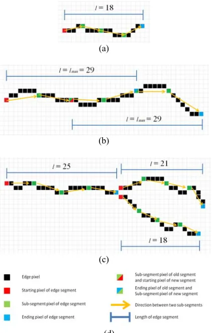
M S S (4) In the conventional Canny technique, only the edge gradient is considered. In addition to that, the proposed technique also considers the length and directional change of the edge. The measurement of the length of the edge is illustrated in Figure 1. The length of the edge in the local maxima image IM is measured from the starting
5106 diagonal. The measurement of the edge length also considers edge with branches. A line segment with a length of 29 pixels, lmax is used to track the edges.
If edge is shorter than the line segment, the length of the edge, l is measured form the starting pixel to the ending pixel of the edge as shown in Figure 1a. If the edge is longer, the line segment scans, like a moving window, the entire length of the edge. In order to ensure the smoothness of the edge measurement, the line segment moves halfway of its size as shown in Figure 1b. If the edge has branches, the edge is divided into three or more edges from the branch points and each edge branch is treated as new edge and its length is measured in a similar fashion either the edge is shorter or longer than the line segment, lmax. This procedure is
performed on all edges in the image to generate a length image, IL.
(a)
(b)
(c)
[image:3.612.91.302.311.642.2](d)
Figure 1: Edge segmentation. (a) Short edge, (b) long edge and (c) edge with branches (d) legends.
In order to measure the directional change, each edge segment is divided into four sub-segments with equal length. Each sub-segment has a direction, θ ranging from 0 ≤ θ < 2π. The
directional change between two sub-segments Δθk
is calculated using Equation 5, where k = (1, 2, 3) and 0 ≤ Δθk < π. As a result, each segment has three
directional changes Δθk. If the edge segment has
branches, additional directional change, Δθb = π is
included, otherwise Δθb = 0. Finally, directional
change of the segment, d is calculated using Equation 6, where 0 ≤ d ≤ 1. The higher value of d, the straighter the edge. This procedure is performed on all edges in the image to generate a directional change image ID.
k min
d , d 2 ,
d 2
(5)where
d
k k13 1
3 1
1 1
4 3 4
k b
k
d
(6)All the three edge features: gradient, m; length, l; and directional change, d are scaled using a non-linear sigmoid function as given in Equation 7 and shown in Figure 2. The sigmoid function provides soft tolerance to the features at the thresholding point instead of using a hard on/off step function. Here, the features, m, l and d are represented by variable x in Equation 7.
2 11 1 w x
h x
e
[image:3.612.325.516.438.632.2] (7)
Figure 2 : Sigmoid function
The variable w in Equation 7 is set to 4 in order to get three equal parts (off, transferring, and on) from the second order derivative of the sigmoid function as shown in Figure 3. The variable x in Equation 7 is rescaled using non-linear scaling xp. If x 0.5,
5107
ln 0.5 ln p
t
(8)
and
0.5
2 1
1 ,
1 P
x w x
H x t
e
(9)
where t is the threshold of the function.
If x > 0.5, then
ln 0.5 ln 1 p
t
(10)
and
0.5 2 1 1 1
1 ,
1
P
x w x
H x t
e
[image:4.612.118.523.66.470.2](11)
Figure 3: Second order derivative of the sigmoid function.
The ranges of the threshold values, t on the sigmoid function is shown in Figure 4.
Figure 4: Ranges of threshold, t from 0.1 to 0.9.
Equation 9 and 11 are the basis for the generation of three functions: function HM(IM, tM)
is used to detect edges from the local maxima image, IM, while functions HL(IL, tL) and HD(ID, tD)
are used to remove noises in the length image, IL
and directional change image, ID, respectively. tM,
tL, and tD are the thresholds of the gradient, length,
directional change, respectively. The threshold parameters of the proposed algorithm are determined using a procedure similar to CED in determining the threshold. The gradient threshold tM is determined based on the high threshold value
in the hysteresis step in Canny [6]. The value of thresholds tL and tD are determined from the
histograms of the images IL and ID, respectively.
(a) (b) (c)
(d) (e) (f)
[image:4.612.89.292.101.463.2](g) (h) (i)
Figure 5: Example of edge detection of the proposed algorithm. (a) ‘Cameraman’ image with Gaussian noise. (b) Vertical derivative component. (c) Horizontal derivative component. (d) Magnitude/gradient. (e) Local maxima. (f) Edge gradient feature. (g) Edge length feature. (h) Edge directional change feature. (i) Edge image.
Finally, all the three functions, HM, HL, and
HD, are combined to generate an edge image, IE as
given in Equation 12. The emphasis of each function can be controlled by multiplying them with weights. The weight of the HM function, kM is
set to 50%, while the weights for the HL and HD
functions, kL and kD, are set to 25% each. tE is the
threshold for the edge image, IE that determines
whether the pixel is edge or background. The minimum condition for the edge to pass the three sigmoid functions HM, HL and HD required that HM
[image:4.612.317.520.227.469.2]= 1, which is at the maximum of the “on” part of the second derivative of the function as shown in Figure 2, and the other two functions, HL ≥ 0.2 and
[image:4.612.104.288.514.656.2]5108 the transferring part. Based on these conditions and the weights of the functions, the minimum passing condition was set to tE = 0.6. Figure 5 illustrates
stages of the proposed edge detection applied on a ‘Cameraman’ image degraded with Gaussian noise.
1, 0,
M M L L D D E
E
M M L L D D E
k H k H k H t
I
k H k H k H t
(12)
3. RESULTS
Images that are used in the analyses include synthetic and natural images. These images contain varying degrees of contrast, length, and shape of the edges. For each image, three types of noise: Gaussian, speckle and salt & pepper are added. Results of several edge detectors like CED, EGT, SMC, NLFS, RKT, and the proposed algorithm are compared. These algorithms are selected for the comparison based on the literature. Each algorithm has a different method to handle noise which can help in the comparison of this study. For example: CED reduces noise using Gaussian filter, removing non maxima edge then applying hysteresis thresholding. EGT handles noise using pseudo image generated from Canny then applying receiver operating characteristics thresholding. SMC applies multiple scales of Canny to hand noise as noise does not likely to appear in all scales. NLFS is non-linear edge detection which is robust to impulse noise and RKT is an example of using a large kernel.
Quantitative assessment is done using precision, recall, accuracy, and F1 value, which all of them are based on true positive (TP), true negative (TN), false positive (FP), and false negative (FN) as in Equations 13-16.
TP Precision =
TP+FP (13)
TP Recall =
TP+FN (14)
Accuracy = TP+TN
TP+TN+FP+FN (15)
F1= 2Precision Recall Precision Recall
(16)
For the ‘Letters’ image in Figure 6, the first row shows the image without noise and results of several edge detection techniques, and the second rows shows the image degraded with Gaussian noise and the edge detection results. Third
row shows the image degraded with speckle noise and the results, while the forth row shows the image degraded with salt & pepper noise. The purpose of the analysis on the image without noise is to evaluate the performance of the edge detectors to detect edges in low contrast situations, like letters ‘B’ and ‘E’, and also the boundary of boxes of letters ‘L’, ‘O’, and ‘P’. Only the proposed edge detection technique is able to detect all the edges including letters ‘B’ and ‘E’ as well as boxes of letters ‘L’, ‘O’, and ‘P’. Analysis on the noisy images demonstrated that the proposed technique is able to suppress the noise as well as detect the edges. Figure 7 shows results on the ‘Circles’ image without noise (first row) and with Gaussian noise (second row), speckle noise (third row), and salt & pepper noise (fourth row). Here, the proposed edge detection technique demonstrated its superiority in detection low contrast edges like the outermost circle and less sensitive to noise. The average F1 value, accuracy, precision and recall measured from the two synthetic images are presented in Tables 1-4. Figure 8 shows F1 values measured for ranges of standard deviation for the Gaussian, speckle, salt & pepper noises. In general the proposed technique produced the best results.
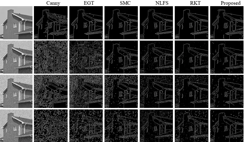
Besides the synthetic images, two natural images are used. Figure 9 shows the ‘Cameraman’ image and Figure 10 shows the ‘House’ image. These images contain long, short, straight, curvy, irregular edges. The performance of edge detection algorithms is evaluated under different conditions, such as, without noise, with Gaussian, speckle, and salt & pepper noises. Results of edge detection techniques on the natural image are difficult to assess quantitatively because derivation of a ground truth image is difficult and subjective to users. Therefore, analysis on the natural image is only performed qualitatively. The proposed edge detection technique produced better results when compare to the other five techniques as it is able to detect low contrast edges, ignore unwanted edges and high resistance to noises. For example, in the ‘Cameraman’ image, edges at the pocket, hand, and building are well detected and ignoring unwanted texture pattern on the ground. The proposed edge detection algorithm also demonstrated high resistance when noises are included.
trade-5109 off between noise and information compare with others. The source of improvement is by making the algorithm focus on longer and straighter edges as noise less likely to create long and straight edges.
The novelty in this work is how to handle noise in an image. This is done by tracking the edges and considering three edge features then use these features to differentiate between true and false edges. This approach only removes noisy edges and does not affect the non noisy edge. In addition it allows low contrast non noisy edges to be detected.
The advantages of the proposed algorithm are very good at detecting low contrast edges in non noisy images at the same time very resistant to noise. This means low trade-off between noise and information. It is also good at localization following CED method. Limitation of this work might be the speed where in experiments it is found that the proposed algorithm is slower three times than traditional CED due to tracking of the edges. However this time is used to find new features that can be used for further image processing and analysis.
4. CONCLUSIONS
In this paper, a new edge detection technique based on Canny edge technique is proposed by combining three edge features: gradient, length, and directional change. The technique is tested with synthetic and natural images by considering images without noise and different types of noise. From the results and comparisons with other algorithms, the proposed technique is able to detect low contrast edges, ignore unwanted edges and remove noise. The results also demonstrate that the proposed technique is more robust to noises as compare to other established edge detection techniques. The key success of this technique is by incorporating length and directional changes edge features to the Canny edge detector.
In this work, it is clear that incorporating more edge features like length and directional changes besides the gradient helped in detecting true edges and ignoring noise. The proposed algorithm satisfies the criteria of good edge detection which is good at detection, good at localization and highly resistant to noise. This means it has low trade-off between noise and information compare with other methods in the light of literature. Future work will consider incorporating more edge features and demonstrate
it advantages in different environments and applications.
REFRENCES:
[1] Melin, P., Gonzalez, C. I., Castro, J. R., Mendoza, O., and Castillo, O. “Edge detection method for image processing based on generalized type-2 fuzzy logic”, IEEE Transactions on Fuzzy Systems, Vol. 22, No. 6, December 2014, pp. 1515-1525.
[2] Russo, F. and Lazzari, A., “Color edge detection in presence of gaussian noise using nonlinear prefiltering”, IEEE Transactions on Instrumentation and Measurement, Vol. 54, No. 1, February 2005, pp. 352-358.
[3] Pellegrino, F. A., Vanzella, W., and Torre, V., “Edge detection revisited”, IEEE Transactions on Systems, Man, And Cybernetics—Part B: Cybernetics, Vol. 34, No. 3, June 2004, pp. 1500-1518.
[4] Torre, V. and Poggio, T. A., “On edge detection”, IEEE Transactions on Pattern Analysis And Machine Intelligence, Vol. 8, No. 2, March 1986, pp. 147-163.
[5] Wang, S., Sun, S., Guo, Q., Dong, F., and Zhou C., “Image edge detection based on rotating kernel transformation”, Image And Signal Processing (Cisp), 2014 7th International Congress On, Dalian, 14-16 October 2014, pp. 397-402
[6] Canny, J., “Finding edges and lines in images”, Report AI-TR-720, MIT Artificial Intelligence Laboratory, Cambridge, MA, 1983.
[7] Yitzhaky, Y., and Peli, E., “A method for objective edge detection evaluation and detector parameter selection”, IEEE Transactions on Pattern Analysis and Machine Intelligence, Vol. 25, No. 8, August 2003, pp. 1027-1033.
[8] Medina-Carnicer, R., Carmona-Poyato, A., Munoz-Salinas, R., and Madrid-Cuevas, F.J., “Determining hysteresis thresholds for edge detection by combining the advantages and disadvantages of thresholding methods”, IEEE Transactions on Image Processing, Vol. 19, No. 1, January 2010, pp. 165-173.
[9] Bao, P., Zhang, L., and Wu, X., “Canny edge detection enhancement by scale multiplication”, IEEE Transactions on Pattern Analysis and Machine Intelligence, Vol. 27, No. 9, September 2005, pp. 1485-1490.
5110 Machine Intelligence, Vol. 32, No. 2, February 2010, pp. 242-257.
[11] Sri Krishna, A., Eswara, R. B., and Pompapathi, M., "Nonlinear noise suppression edge detection scheme for noisy images", International Conference on Recent Advances and Innovations in Engineering (ICRAIE), Jaipur, 9-11 May 2014, pp. 1-6.
[12] Zhu, S., “Edge detection based on multi-structure elements morphology and image fusion”, Computing, Control and Industrial Engineering (CCIE), IEEE 2nd International Conference On, Wuhan, 20-21 August 2011, pp. 406-409.
[13] Bhateja, V. and Devi, S., “A novel framework for edge detection of micro calcifications using a non-linear enhancement operator and morphological filter”, Electronics Computer Technology (ICECT), 3rd International Conference on, 5, Kanyakumari, 8-10 April 2011, pp. 419- 424.
[14] Jiang, J.-a., Chuang, C.-l., Lu, Y.-l., and Fahn, C.-s., “Mathematical-morphology-based edge detectors for detection of thin edges in low-contrast regions”, IET Image Processing, Vol. 1, No. 3, September 2007, pp. 269-277.
[15] Pawar, K. B., Nalbalwar, S. L., "Distributed canny edge detection algorithm using morphological filter", IEEE International Conference on Recent Trends In Electronics, Information & Communication Technology (RTEICT), Bangalore, 20-21 May 2016, pp. 1523-1527.
[16] Berlemont, S. and Olivo-Marin, J. C., “Combining local filtering and multiscale analysis for edge, ridge, and curvilinear objects detection”, IEEE Transactions On Image Processing, Vol. 19, No. 1, January 2010, pp. 74-84.
[17] Chen, Y., Fang, B., and Wang, P., “An edge detection algorithm based on beamlet transform and its applications”, IEEE Intelligent Vehicles Symposium, Xi’an, 3-5 June 2009, pp. 163-167. [18] Sghaier, M. O., Coulibaly, I., and Lepage, R.,
"A novel approach toward rapid road mapping based on beamlet transform", IEEE Geoscience And Remote Sensing Symposium, Quebec City, QC, 13-18 July 2014, pp. 2351-2354.
[19] Pei, S.-C., and Ding, J.-J., "The generalized radial Hilbert transform and its applications to 2D edge detection (any direction or specified directions)," Acoustics, Speech, and Signal Processing, 2003. Proceedings. (ICASSP '03).
2003 IEEE International Conference on, 3, 6-10 April 2003, pp. 357-360.
[20] Pei, S.-C., Ding, J.-J., Huang, J.-D., and Guo, G-C., "Short response Hilbert transform for edge detection," APCCAS 2008 - 2008 IEEE Asia Pacific Conference On Circuits And Systems, Macao, 30 November-3 December 2008, pp. 340-343.
[21] Golpayegani, N., and Ashoori, A., "A novel algorithm for edge enhancement based on Hilbert Matrix," 2nd International Conference on Computer Engineering And Technology, Chengdu, 16-18 April 2010, pp. V1-579-V1-581.
[22] Wang, B. and Fan, S., "An Improved CANNY Edge Detection Algorithm," Second International Workshop on Computer Science and Engineering, Qingdao, 28-30 October 2009, pp. 497-500.
[23] Biswas, R. and Sil, J., “An Improved Canny Edge Detection Algorithm Based on Type-2 Fuzzy Sets”, 2nd International Conference on Computer, Communication, Control and Information Technology (C3IT-2012), 4, 25-26 February 2012, pp 820-824.
[24] Zhou, P., Ye, W., Xia, Y., and Wang, G., “An Improved Canny Algorithm for Edge Detection”, Journal of Computational Information Systems, Vol. 75, No. 5. May 2011, pp. 1516-1523.
[25] Leordeanu, M., Sukthankar, R., and Sminchisescu, C., “Generalized boundaries from multiple image interpretations”, IEEE Transactions on Pattern Analysis And Machine Intelligence, Vol. 36, No. 7, July 2014, pp. 1312-1324.
[26] Koschan, A. and Abidi, M., “Detection and classification of edges in color images”, IEEE Signal Processing Magazine, Vol. 22, No. 1, January 2005, pp. 64-73.
[27] Lei, T., Fan, Y., and Wang, Y., “Colour edge detection based on the fusion of hue component and principal component analysis”, IET Image Processing, Vol. 8, No. 1, January 2014, pp. 44–55.
[28] Dollar, P. and Zitnick, C. L., “Fast edge detection using structured forests”, IEEE Transactions on Pattern Analysis And Machine Intelligence, Vol. 37, No. 8, August 2015, pp. 1558-1570.
5111 Vancouver BC Canada, 10-13 September 2000, pp. 796–799.
[30] Fu, W., Johnston, M., and Zhang, M., “Low-level feature extraction for edge detection using genetic programming”, IEEE Transactions on Cybernetics, Vol. 44, No. 8, August 2014, pp. 1459-1472.
[31] Qasim, M., Woon, W. L., Aung, Z., and Khadkikar, V., “Intelligent edge detector based on multiple edge maps”, Computer Systems And Industrial Informatics (ICCSII), International Conference on, Sharjah, 18-20 December 2012, pp. 1-6.
5112
Canny EGT SMC NLFS RKT Proposed
[image:9.612.100.509.90.352.2]
Figure 6: Results of edge detection techniques on ‘Letters’ image. Original (first row). Degraded with Gaussian noise (second row), speckle noise (third row), salt & pepper noise (fourth row).
Canny EGT SMC NLFS RKT Proposed
[image:9.612.99.517.404.649.2]5113
Table 1 Average F1 value of the synthetic images.
No
noise Gaussian Speckle
Salt & Pepper
Canny 0.9833 0.5394 0.6271 0.5914
EGT 0.9009 0.5988 0.6438 0.6492
SMC 0.9101 0.6801 0.7208 0.6479
NLFS 0.9515 0.7146 0.7825 0.6966
RKT 0.9121 0.6865 0.6603 0.6077
Proposed 0.9970 0.7328 0.8788 0.6865
Table 2 Average accuracy of the synthetic images.
No
noise Gaussian Speckle Salt & Pepper
Canny 0.9974 0.7632 0.8995 0.8806
EGT 0.9864 0.7704 0.9167 0.8872
SMC 0.9886 0.9023 0.9524 0.9081
NLFS 0.9928 0.9345 0.9605 0.9335
RKT 0.9880 0.9248 0.9441 0.9128
Proposed 0.9995 0.9594 0.9809 0.9498
[image:10.612.311.509.109.190.2]
Table 3 Average precision of the synthetic images.
No
noise Gaussian Speckle
Salt & Pepper
Canny 1.0000 0.3900 0.4849 0.4608
EGT 1.0000 0.4610 0.5308 0.5315
SMC 0.9978 0.6071 0.7146 0.5654
NLFS 1.0000 0.6482 0.7348 0.6161
RKT 0.9961 0.6778 0.6455 0.5444
Proposed 1.0000 0.7456 0.8728 0.6804
Table 4 Average recall of the synthetic images.
No
noise Gaussian Speckle Salt & Pepper
Canny 0.9677 0.9252 0.8933 0.8376
EGT 0.8196 0.9322 0.8204 0.8709
SMC 0.8377 0.8340 0.7369 0.7931
NLFS 0.9076 0.8233 0.8399 0.8171
RKT 0.8415 0.7424 0.6805 0.7058
Proposed 0.9940 0.7220 0.8980 0.6976
(a) (b) (c)
Figure 8 Average F1 value for two synthetic images where sigmas, of the (a) Gaussian, (b) speckle, and (c) salt &
pepper noises were varied.
[image:10.612.104.302.242.327.2] [image:10.612.316.507.244.326.2] [image:10.612.99.513.270.492.2]5114
[image:11.612.90.510.72.336.2]Canny EGT SMC NLFS RKT Proposed
Figure 9: Results of edge detection techniques on ‘Cameraman’ image. Original (first row). Degraded with Gaussian noise (second row), speckle noise (third row), salt & pepper noise (fourth row).
Canny EGT SMC NLFS RKT Proposed
[image:11.612.92.507.401.643.2]