The development of analysis of variance techniques for angular data

(1)

The development of analysis of variance techniques for

angular data.

HARRISON, David.

Available from Sheffield Hallam University Research Archive (SHURA) at:

http://shura.shu.ac.uk/19759/

This document is the author deposited version. You are advised to consult the

publisher's version if you wish to cite from it.

Published version

HARRISON, David. (1987). The development of analysis of variance techniques for

angular data. Doctoral, Sheffield Hallam University (United Kingdom)..

Copyright and re-use policy

See

http://shura.shu.ac.uk/information.html

(2)

65 O

(3)

ProQuest Number: 10697061

INFORMATION TO ALL USERS

The quality of this reproduction is dependent upon the quality of the copy submitted.

In the unlikely event that the author did not send a com plete manuscript and there are missing pages, these will be noted. Also, if material had to be removed,

a note will indicate the deletion.

uest

ProQuest 10697061

Published by ProQuest LLC(2017). Copyright of the Dissertation is held by the Author.

This work is protected against unauthorized copying under Title 17, United States C ode Microform Edition © ProQuest LLC.

ProQuest LLC.

789 East Eisenhower Parkway P.O. Box 1346

(4)

THE DEVELOPMENT OF ANALYSIS OF VARIANCE TECHNIQUES

FOR ANGULAR DATA

DAVID HARRISON

A thesis submitted to the Council for National Academic Awards in partial fulfilment of the requirements for the degree of Doctor of Philosophy

Sponsoring Establishment

Department of Applied Statistics and Operational Research Sheffield City Polytechnic

(5)

(6)

TH E DEVELOPMENT OF ANALYSIS OF VARIANCE TECHNIQUES FOR

ANGULAR DA TA

D HARRISON

ABSTRACT

In many areas of research, such as within medical statistics, biology and geostatistics, problems arise requiring the analysis of angular (or directional) data. Many possess experimental design problems and require analysis of variance techniques for suitable analysis of the angular data. These techniques have been developed for very limited cases and the sensitivity of such techniques to the violation of assumptions made, and their possible extension to larger experimental models, has yet to be investigated.

The general aim of this project is therefore to develop suitable experimental design models and analysis of variance type techniques for the analysis of directional data.

Initially a generalised linear modelling approach is used to derive parameter estimates for one-way classification designs leading to maximum likelihood methods. This approach however, when applied to larger experimental designs is shown to be intractable due to optimization problems.

The limited analysis of variance techniques presently available for angular data are reviewed and extended to take account of the possible addition of further factors within an experimental design. These are shown to breakdown under varying conditions and question basic underlying assumptions regarding the components within the original approach.

A new analysis of variance approach is developed which possesses many desirable properties held in standard 'linear' statistical analysis of variance.

(7)

ACKNOWLEDGEMENTS

I would like to express my gratitude to Dr G K Kanji, acting Head of Department,

and Dr R J Gadsden, Principal Lecturer, for introducing me to this field and under

whose supervision and constant encouragement this work has been carried out. I

would also like to thank the members of the Departments of Mathematics and

Statistics for their assistance on specific points.

My indebtedness to the work of Professor K V Mardia will be evident; I should

here like to thank him, in addition, for his valuable comments and suggestions.

I wish to thank Ms Ann Moon for the excellent typing of this thesis produced from

the demanding material with which she had to work.

Finally, and most of all, I would like to express my love and gratitude to my wife

(8)

x 2

Distributions for the

Randomised Block Design and the Two-way Classification

and their Corresponding F Statistics 98

6.5 Summary 114

(11)

-CHAPTER 7

THE ROBUSTNESS AND POSSIBLE COLLAPSE OF TH E EXTENDED

TECHNIQUES

7.1 Introduction 115

7.2 Robustness of Assumptions 115

Example 7.2.1

7.3 A Further Approach to Watson and Williams Design Using a

Regression Model 119

7.3.1 Total Measure of Variation 122

7.3.2 Residual or Within Measure of Variation 123

7.3.3 Between Measure of Variation 124

7.3.3.1 Combining Mean Angular Directions and Resultant

Lengths 125

7.4 Cross Product Terms and the Analysis of

Cross-Classification 130

7.5 Summary 134

CHAPTER 8

DEVELOPMENT OF A NEW ANALYSIS OF VARIANCE PROCEDURE

8.1 Introduction 135

8.2 Minimising Chord Distances to Build New Model Components 135

8.2.1 Total Measure of Variation 136

8.2.2 Residual Measure of Variation 138

8.2.3 Between Measure of Variation 139

(12)

8.4 Analysis of Cross-Classification and Interaction 143

8.4.1 The Interpretation of Interaction on the Circle 143

8.4.2 The Calculation of Interaction on the Circle 147

8.5 Other Design Models 151

8.5.1 The Randomised Complete Block Design 151

8.5.2 Latin Square Design 152

8.5.3 Nested or Hierarchical Design 154

8.5.4 Three-way Classification 155

8.6 Summary 156

CHAPTER 9

TH E DISTRIBUTION OF THE NEW COMPONENTS A ND TEST

STATISTICS

9.1 Introduction 157

9.2 Small Concentration Parameter, k 158

9.3 Large Concentration Parameter, k 160

9.3.1 Distribution of fc(N-(C2/N)) 161

9.3.2 Distribution of fc((R2/N )-(C 2/N)) 162

9.3.3 Distribution of fc(N-(R2/N)) 162

9.4 The Variance of the Component Chi-Squared Approximations 163

9.4.1 Variance of (N -(R 2/N)) 163

9.4.2 Variance of (N-^(R2j/N 2j)) 166

9.4.3 Variance of ® R 2j/N j)-(R 2/N)) 167

9.5 The Adequacy of the New Procedure, for Large k 168

9.6 Comparing the Power of the Tests, for Large k 184

9.7 The Adequacy of the New Procedure, for Small k 187

9.8 Comparing the Power of the Tests, for Small k 191

9.9 Summary 194

(13)

-CHAPTER 10

TH E RANDOMISED COMPLETE BLOCK AND T W O -W A Y DESIGNS

V IA TH E NEW APPROACH

10.1 Introduction 196

10.2 Randomised Complete Block and Two-way Classification with

Interaction Designs, for Large k 196

10.3 Accuracy of the Associated \ 2 Approximations for the Randomised Complete Block and the Two-way Classification

Designs with their Corresponding F Statistics, for

Large k 200

10.3.1 The Randomised Complete Block Design 200

10.3.2 Two-way Classification with Interaction 211

10.4 Randomised Complete Block and Two-way Classification with

Interaction Designs, for Small k 218

10.5 Accuracy of the Associated Chi-squared Approximations for

Small k 219

10.6 Summary 227

CHAPTER 11

ANALYSIS OF VARIANCE EXAMPLES FOR CIRCULAR STATISTICS

11.1 Introduction 228

11.2 One-way Analysis 228

Example 11.2.1 for Large k Example 11.2.2 for Small k

11.3 Randomised Complete Block Design 234

(14)

11.4 Two-way Classification with Interaction

Example 11.4.1 for Large k Example 11.4.2 for Small k 11.5 The Latin or Graeco-Latin Square

Example 11.5.1

11.6 Split Plot Design

Example 11.6.1

11.7 Summary

CHAPTER 12

SYNOPSIS OF RESULTS AND CONCLUSIONS

Appendix A

Index of Notation

Appendix B

The Simulation and Accuracy of Numerical Results

(15)

CHAPTER 1

INTRODUCTION

1.1 Directional Data

In many scientific fields the experimenter is interested primarily in the direction of a

measured variable. These observations will be bearings from some central point, or

origin, ending on a sphere or circumference of a circle, and may be regarded as

vectors. The radius can be represented as a unit vector, while the length or

magnitude of the vector is not important. Directions may be thought of in any

number of dimensions but in practice they are invariably collected in two or three

dimensional space. The tests and new results presented in this thesis are solely

concerned with directions in two-dimensions. Directions are measured by angles

ranging from 0* to 360*, or, equivalently, from 0 to 2x radians. Circular or

directional data is the name given to data which arise when the observations are

angles.

There are many examples of circular data originating from various disciplines. For

example, geologists study the orientation of fractures in deformed rocks to interpret

structural changes, and the orientation of cross-bedding or particles in undisturbed

sediments to the direction of depositing currents of wind and water. (Pincus (1953),

Curray (1956), Sengupta and Rao (1966), and Sanderson (1976)). The classic example

of directional data is from the study of bird orientation in homing or migration

which involves observing the birds vanishing angles from their release point.

Zoologists use such data to investigate consistency of bird migration under certain

conditions. Many examples from this field of study are well cited and illustrated by

Batschelet (1965, 1981).

(16)

-Directional data is not confined to observations directly measured in degrees or

radians, but may also occur in the area of biological rhythms. A period of 24 hours

corresponds to a full turn of 360 degrees. Similarly, a month, a year or any other

period of a cyclic event may be represented by a rotation of 360 degrees. The

number of deaths due to a disease or the number of onsets of a disease in each

month over years fall in this category and can be treated as directional or circular

data. Other examples of this type can be seen in Gumbel (1954).

It is tempting to use the conventional measures of location and spread used in linear

analysis to analyse directional data. For example, suppose our data are the four

values 5, 14, 351 and 10, a simple arithmetic mean would give a value of 95. For

linear analysis this is understandable as the value of 351 has a large influence and

draws the mean away from the other data points. If these values are now regarded

as angles the spread of the whole sample is reduced, since in angular terms the

sample value of 351* is now situated close to the other data points. Similarly the

point of central location will have changed considerably and can now be seen to be

around zero degrees. Then the simple arithmetic mean would not, in general, give a

meaningful mean direction of the sample, similarly, the standard deviation would not

give a good measure of dispersion. If, however, the zero direction was taken at a

different position on the circle such as the y-axis in place of the x-axis then the

linear measure may give a sensible result. For example, if the above sample values

were rotated by 90*, to become 95*, 104*, 81* and 100*, the arithmetic mean would

give a sensible result of 95*. It is therefore not possible to define an arithmetic

mean or standard deviation in such a way that it is invariant under a rotation of the

circle. This heavy dependence on the zero direction shows the inappropriate use of

basic linear methods for circular statistics. Simple examples of such problems are

given by Batschelet (1965, 1981), Mardia (1972) and Watson (1983). Distribution

functions, characteristic functions and moments all suffer from the same draw-back

and must in some way take account of the natural periodicity of the circle.

(17)

-1.2 A General Thesis Review

Having introduced the study of directional data, this section gives a brief review of

the work discussed within each of the following chapters, whilst indicating the

structure and progression of the thesis as a whole. The following two sections within

this chapter give further background to the subject of directional data. The first

discusses different types of probability distributions that may exist on the circle, whilst

the second states the elementary statistics of angular data required for further use in

later chapters.

In Chapter 2 the von Mises distribution is discussed from estimation and distributional

view points. The maximum likelihood estimates of the von Mises parameters are

seen to be asymptotically independent so that construction of simple large-sample

tests, for differing hypotheses regarding the parameters, may be carried out. Interest

is focused on the distributional form of the resultant length on the random (Uniform)

distribution, k - 0, and the von Mises distribution. The results from the special case of the random distribution are required since terms in its solution arise again in

the general distribution theory. A summary of exact and approximate moments of

the resultant length, R, are given in preparation for the derivation of further circular

statistical tests.

Chapter 3 is a review of the maximum likelihood results and tests for the von Mises

distribution. Extensive investigation of the many approximations for the von Mises

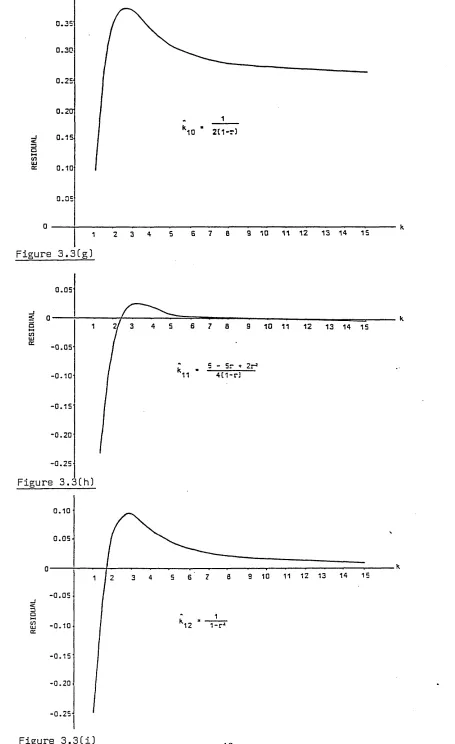
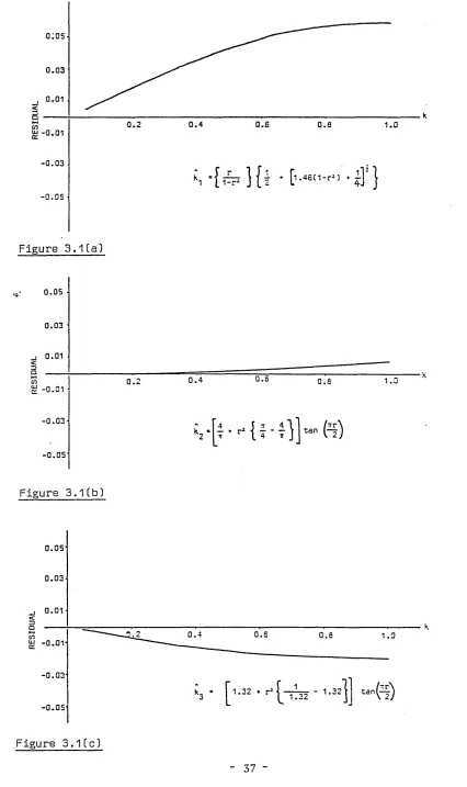
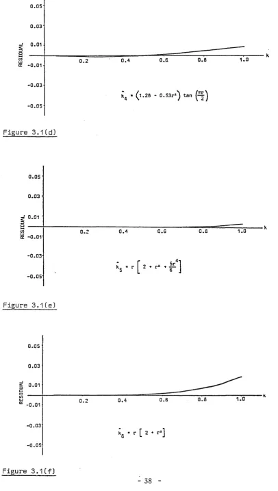
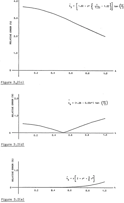
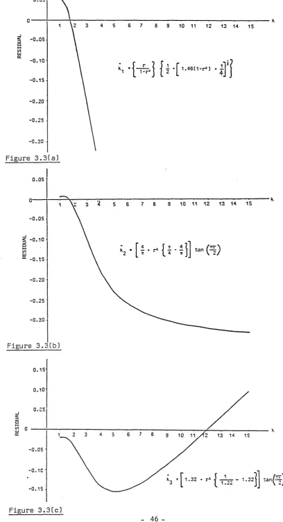
concentration parameter, k, for both small and large k, has been undertaken. Seven approximations for the maximum likelihood estimate of small k, k, which have been cited by various authors are reviewed. Their corresponding values, residuals and

relative residuals are plotted to enable comparison and evaluation of their accuracy.

A

Similar work is carried out for nine approximations to large k, k. A summary of the 'best' and 'best simple1 approximations is given in Section 3.5 against varying

(18)

-ranges of the concentration parameter.

Chapter 4 gives an historical review of the development of analysis of variance

techniques. The work covers the exact and approximate tests for differing mean

directions derived by Watson (1956), Watson and Williams (1956) and Stephens

(1962a, b and c), to multi-sample tests for the equality of concentration parameters.

The homogeneity tests for varying ranges of concentration parameter are cited for

later use with new design tests.

Chapter 5 discusses the use of the generalised linear modelling approach for circular

statistics to derive parameter estimates leading to maximum likelihood methods. For

circular statistics it is shown to be desirable to choose the constraint on the angles

specifying the factor parameters so that their sines sum to zero. Section 5.3 shows

how parameter estimates for the one-way classification design may be found and

therefore assist in further understanding of the underlying structure under

investigation. The approach, however, when applied to larger experimental designs is

seen, at this time, to be intractable since the optimization procedures cannot be

solved due to the numerous local maxima found within the constrained equations.

Chapters 6 and 7 examine the possibility of extending the original procedure for the

one-way analysis, derived by Watson and Williams (1956), to larger designs, for large

k. Chapter 6 shows the construction of the nested or hierarchical design, the randomised complete block and two-way classification design with interaction together

with a comparison of their accuracy to the chi-squared and F distributions. Chapter

7, however, shows the possible collapse of these test statistics under particular

circumstances. The problems associated with the combining of circular mean

directions are shown to be influential in this collapse whilst the cross-product terms

are seen to be non-zero and requiring a correction factor to eliminate them.

(19)

-Chapter 8 develops a new analysis of variance approach by taking account of the

resultant lengths together with their corresponding mean directions to eliminate the

possible collapse discussed in Chapter 7. The method is still based on maximum

likelihood techniques but requires the user to test for equality of concentration

parameters prior to testing for any difference between mean directions. The

cross-product terms are examined and found to equal their desired combined value of

zero. An investigation of the interpretation and representation of interaction on the

circle is given in Section 8.4 prior to its calculation via the new approach. For the

two-way design the cross-product terms are again shown to equal zero. Further

designs are then constructed in the same manner.

Following the development of the procedures in Chapter 8, Chapter 9 examines the

statistical theory and distributions behind the new design components and test

statistics. The exact theoretical distributions are seen to be intractable, and therefore

distribution approximations are used to examine the theory whilst simulation

techniques reproduce the distributions of the test statistics for comparison with their

assumed expected distributions. The comparisons are carried out for both large and

small k and test statistic improvements are made using the component moments. The power of the new tests are also compared with existing tests for the

multi-sample case and are seen to compare favourably for both large and small k.

Chapter 10 reproduces the components within the new procedure for the randomised

complete block and two-way designs together with their improvement factor derived

in Chapter 9. The component statistics and test statistics are compared to their

respective exact chi-squared and F distributions. These two designs are used to

illustrate the validity of the approach for larger more complex design situations.

(20)

-Chapter 11 gives several examples where the new approach is applied to real data

sets with varying sizes of concentration parameter. The examples vary from the

one-way design to the Graeco-Latin square and split plot designs.

Finally Chapter 12 summarises the development of the new analysis of variance

techniques. The adequacy of the new procedures, produced for both large and small

concentration parameter, are discussed together with their respective components and

test statistics.

Appendix A gives a list of notations used throughout the thesis together with the

design notations set out in tabular form. Appendix B reviews the techniques used to

simulate the von Mises distribution and the required experimental designs. The size

and accuracy of the numerical results are also discussed.

1.3 Probability Distributions on the Circle

There is no single distribution on the circle which has all the desirable properties

which the Normal distribution possesses on the line. Most of the distributions on the

circle have been derived either from transformations of the standard univariate (or

bivariate) distributions or as circular analogues of important univariate characteristics.

Linear distributions may have a finite range, range to infinity, or may even extend

over the whole straight line. Circular distributions, however, are always finite

ranging from 0* to 360’ (or, equivalently, 0 to 2ir), or are fractions within this

range.

In general, circular distributions are continuous over the circumference of the circle

and may be specified by a probability density function f(0), which is a periodic

function satisfying

(21)

-" 27T

f ( 0 ) d0 - 1 ( 1 . 3 . 1 )

. o

Although no circular distribution holds all the desirable properties seen in the Normal

distribution, the von Mises distribution (originally referred to as the Circular Normal

distribution) is the most generally used distribution in statistical inference on the

circle. The importance of the von Mises distribution on the circle is often compared

to that of the Normal distribution on the line.

The distribution has probability density function

f ( 0 ) = 2ffT (E) exp^ cos( 6 ~ Mo)l 0 < 6 < 2x ( 1 . 3 . 2 )

where I 0(fc) is a modified Bessel function, and A: is a parameter of concentration of

the data about a mean direction nQ. A complete discussion of the von Mises and its properties can be seen in Chapter 2.

There are two limiting cases of circular distributions. The first case occurs when all

the angles are the same i.e. concentrated at one single point 8 = fiQ. The 'point' distribution has little if no practical or theoretical interest here, but has been used

for the analysis of Brownian movement and the paths of beta rays.

The second limiting case is the Uniform distribution, where every angle on the unit

circle has an equal chance of occurring or no sector is preferred to any other sector.

The probability density of 6 is constant over the whole circumference and is defined by

f ( 0 ) = 0 < 8 < 2tt ( 1 . 3 . 3 )

As there is no concentration of points about any given direction on the circle, then

no mean direction exists. Polya (1935) used an analogue of this when he investigated

whether the stars are distributed at random over the celestial sphere.

(22)

-As in the linear case an infinite number of circular distributions exist. Among these,

a few, possessing some desirable properties, have received attention. After the von

Mises, probably the most important is the wrapped Normal distribution. This

distribution is a natural conversion of the Normal distribution and is obtained, as its

name suggests, by wrapping the Normal distribution around the circumference of the

circle and adding those probabilities that fall into the same sector of the circle. The

addition of the overlapping tails leads to a rather complicated density function,

though when cr is small the distribution will be approximately Gaussian in (0,2k). Like the Circular Uniform distribution the wrapped Normal distribution possess the

additive property i.e. the sum of two or more wrapped Normal distributions produces

another wrapped Normal distribution with related parameters. The probability density

of a random variable 0, with mean angle /i0 = 0* , from the wrapped Normal

distribution is

f ( 0 ) --- — T exp[~(<> t A m ) 2 ] o < e < 2x ( 1 . 3 . 4 ) O' V 2 7 1 _n=-ooL 1 2<r 1

where the mean vector length is

- c r2 exp

As p tends to zero, the wrapped Normal distribution approaches the Uniform

distribution, and as p tends to one it is concentrated at a single point. The

distribution has applications in the study of diffusion processes, and amongst others

has been examined by Stephens (1963) and Bingham (1971).

Another distribution which has been wrapped around the circle in a similar manner

to the Normal is the Cauchy distribution. The result is again a unimodal and

symmetric circular distribution possessing the additive property. With mean angle fiQ and mean vector length p the probability density function for the wrapped Cauchy is

(23)

-introduced by Levy (1939) and studied by Wintner (1947).

Other circular distributions of less importance include the cosine distribution, also

called the sine wave distribution, with mean vector length p and mean angle p 0, and

has the density function

f ( 0 ) — 7s— + — cos(0 - p 0) ( 1 . 3 . 6 )

Ztt tt

and the cardioid distribution with the density function

f ( 0 ) - [1 + 2p cos(0 - (iQ)] ( 1 . 3 . 7 )

introduced by Jeffreys (1948).

All the circular distributions discussed so far have been unimodal distributions, with a

single preferred direction of p Q. There are, however, circular distributions with multimodal directions. (1.3.8) gives the density function of a multimodal von Mises

distribution where v denotes the number of modes.

f (0) = 2^1 (k) exP ^ cos v ( 0 " ^o)3 ( 1 . 3 . 8 )

This was suggested by Breitenberger (1963) and further investigated by Stephens

(1965).

Many examples of bimodal data can be found, particularly in scientific fields where

orientation is measurable but direction is not. Batschelet (1965, 1981) gives many

examples of bimodal data from animal orientation and navigation. A similar situation

occurs if we observe the position of undirected straight lines or undirected axes.

(24)

removal of their electric charge. These particles do not have a 'head' or 'tail' and

so the observations lie in the range 0 to x radians.

Other unimodal circular distributions were discussed by Mardia (1972 p.48-61).

Batschelet (1981 p.275-90) also reviews skewed, flat-topped and sharply peaked

circular distributions.

The most widely used circular distribution, however, is the von Mises distribution and

it is on this distribution that this thesis is based. The following chapters investigate

and extend the theory and uses of this distribution.

1.4 Statistics of a Circular Distribution

As we noted in Section 1.1 the simple arithmetic mean would not, in general, give a

meaningful mean direction of a sample of angles 0 1> e 2, ...., %• The mean direction in circular statistics is determined by applying trigonometric functions.

Let Pj be one of the N observed angles 0j, i = 1, 2,...,N , with origin 0. Let q

and S[ be the rectangular components of Pj. Then by definition of sine and cosine,

c j = cos 0j sj = s in ( 1 . 4 . 1 )

where

N N

( 1 . 4 . 2 ) i =l

Therefore, if R is the length of the resultant vector with components

mean direction, with components C and S, then

r = (C 2 + S2) 2 ( 1 . 4 . 3 )

N N

R - Nr ( 1 . 4 . 4 )

(25)

-Applying basic trigonometry to calculate 6, the mean direction of the sample

arc tan

180 + arc tan

i f C > 0

i f C < 0

with the exceptional cases of

90* i f C = 0 and S > 0

270* i f C = 0 and S < 0

undetermined i f C - 0 and S = 0

Figure 1.4.1 illustrates these circular measures:

( 1 . 4 . 5 )

( 1 . 4 . 6 )

uni

= Sin 0£.

Cc = coS

Oc

Figure 1.4.1 The Circular Statistics

[image:25.612.57.525.46.697.2]

(26)

-It is clear from Figure 1.4.1 that the length of the resultant cannot exceed N and

similarly, from (1.4.4), that r cannot exceed 1.

Hence,

In the extreme case when all sample points fall onto the same point, the length of

the mean vector, r, equals 1. When points are close together, concentrated over a

small arc, the centre of mass is still very close to the circumference of the unit

circle, and r is close to 1. Less concentration leads to smaller values of r. At the

lower end r = 0, with no concentration around a single direction. Hence, in

unimodal samples, the mean vector length, r, serves as a measure of concentration.

From the above results we may now see that 6 has some desirable properties as a measure of location. One such property is that the mean vector does not depend on

the zero direction of the sample. If a rotation of \p is applied to each angle, then the sample values 6\ turn into 6[ = 6\ - \p. Similarly the new mean angle is

6" = 6 - \p, but the mean vector length, r, remains invariant.

Examining the sine of the difference between the mean angular direction and the

sample angles, it is easily shown that

( 1 . 4 . 7 )

and

( 1 . 4 . 8 )

N

d . 4 . 9 ) i =l

which is analogous to

N

( 1 . 4 . 1 0 )

in linear statistical analysis.

(27)

-Similarly, for the cosine of the difference

N

J cos(6{ - 6) = R ( 1 . 4 . 1 1 )

i =l

and therefore

N

i T 2[1 - cos( 9 j - ? ) ] - 2(1 - r ) ( 1 . 4 . 1 2 ) 1=1

For small deviations, 6\ - 6

2[1 - cos( 0 j - 0)] « ( ei - I ) 2 ( 1 . 4 . 1 3 )

hence,

N

1 J (« i - 9 ) 2 * 2(1 - r ) ( 1 . 4 . 1 4 )

i= l

which is analogous to

N

i ^ (X | - x ) 2 = s 2 ( 1 . 4 . 1 5 )

i =l

in linear statistics.

Equation (1.4.12) may be defined as the angular variance and, from (1.4.14), is

asymptotically equivalent to the variance in linear statistics.

Taking the square root of (1.4.12) gives a measure of dispersion, equivalent to the

standard deviation

s = [2(1 - r ) ] i ( 1 . 4 . 1 6 )

called the mean angular deviation.

(28)

-The basic results of this section were adapted from Batschelet (1981) where further

discussion of the properties are given. The analogies have been reiterated here so

further use may be made of them in later chapters.

(29)

-CHAPTER 2

TH E VON MISES DISTRIBUTION

2.1 Derivation

Gauss showed that the Normal distribution can be derived by the method of

maximum likelihood with the single assumption that the mean is the most probable

value. Von Mises (1918) applied this to a circular variate, and for this reason

Gumbel, Greenwood and Durand (1953) referred to the distribution as the Circular

Normal Distribution. Von Mises procedure was for a distribution f(0| - n 0), such that the direction fiQ upon N observations 0 lt 0 2, ... 0^ is a maximum given by the constraints

where f(0) is the required distribution and f'(0) is the first derivative of f(0) with

respect to n Q. Since the equations (2.1.1) and (2.1.2) are identical for each 0j, therefore

N

(

2

.

1

.

1

)

i= l

and

(

2

.

1

.

2

)

f ' ( * - Mo)

---sin(0 - /t0) f (0 - H0)

( 2 . 1 . 3 )

The equation has the solution

f(0 - ji0) - U exp[/c cos(0 - /i0) ] ( 2 . 1 . 4 )

where the two variables U and k are linked by the condition (1.3.1).

(30)

-Hence

U - 1

exp[k cos(6 - nQ) ] d(0 - /tQ) o

1 _{( 2 . 1 . 5 )}

2x10(k)

where 10(k) is the modified Bessel function of the first kind and order zero. A proof of (2.1.5) can be seen in Mardia (1972, p.58).

The von Mises distribution then, denoted as M (/*0,fc), is given by

The von Mises distribution is unimodal and symmetric with its mode at fiQ and anti-mode at n Q + x. For k=0, the von Mises degenerates into the Uniform distribution, and for large k the distribution concentrates around the mean direction. Therefore, k is called the parameter of concentration. The concentration parameter k is analogous to the inverse of the variance parameter cr2 of the Normal distribution in its effect on the shape of the distribution. For sufficiently large k we may approximate the von Mises by the Normal distribution. Using an approximation

quoted by Bickley (1957), for large k

2x10(k) exP ^ cos(0 “ *o>]

(

2

.

1

.

6

)

2.2 Properties of the von Mises Distribution and its Parameters

1 exp(k) 10c « - — ---(2r k ) i ( c( k ) )

where

( 2 . 2 . 3 )

Gumbel, Greenwood and Durand (1953) simplified (2.2.3) to obtain

M(0,

k)

» N ( 0 , / H )

alternatively

0 V F « N( 0,1) ( 2 . 2 . 4 )

Upton (1974) considered more accurate approximations by taking further terms in the

power series of ((cos 0) - 1), and produced two new approximations

v / F 0 » N ( 0 ,1) ( 2 . 2 . 5 )

and more accurately,

J T 1

-8k 241 1 + 4k 03 « N ( 0 , 1)

_')■

(

2

.

2

.

6

)

A fourth approximation was considered by Upton (1974) given by Mardia (1972,

p.64), without proof;

i

0 « N ( 0 , 1) ( 2 . 2 . 7 )

Upton tested the power of all the approximations, finding that all four consistently

overestimated the upper tail probability. Approximation (2.2.6) was found to be the

best, and this was later confirmed from further work by Hill (1978).

Stephens

(32)

-(1962c) gave another approach to the equality of the two distributions using the

moment generating function.

Estimates of the parameters k and /x0 may be obtained by means of the maximum likelihood method.

A sample of N angles •••% are collected from a von Mises distribution with

unknown population parameters k and pL0 which we wish to estimate. The probability density for these angles is

CN exp[/c cos(0 1 - /*0) ] exp[/c cos(0 2 - /*0) ] ...

- CN exp k[cos(6^ - /i0) + cos(0 2 - fiQ) + (2 .2 . 8)

where

1

2x10(k)

The log likelihood function is

N

log L(fi0 ,k) - -N log 10(k ) + k ^ cos(0j - /i0) + const i= l

( 2 . 2 . 9 )

For the maximum likelihood estimate of the parameter (i0

“ k [ s i n ( 6 , - n 0) + s in(02 - fLQ) +

N

(

2

.

2

.

10

)

a

and vanishes for the particular value (nQ) with

N

(33)

-From (1.4.yj we Know mat mis equauon is sausriea ior me sampie mean angie a which we calculated in (1.4.5). Hence, the maximum likelihood estimate of the

parameter p Q of a von Mises distribution is the sample mean angle 0. Bingham and Mardia (1975) showed that there exists only one circular distribution for which the

sample mean angle is the maximum likelihood estimate of the population mean angle,

namely the von Mises distribution.

For the maximum likelihood estimate of the parameter k

N

dlog L 1,(10

N

---d(/c) I 0(k) + ^ c o s ( 0 { -

H0)

( 2 . 2 . 1 1 )

Therefore dlog Ud{k) is zero if

N

- £ cos( 0 j - IX0) ( 2 . 2 . 1 2 )

I 00 0 N ^

The right hand side is the mean vector length of the sample, r, as indicated by

equation (1.4.11). Hence, the maximum likelihood estimate of k is the solution of

I , < £ ) R

A ( k ) --- r ( 2 . 2 . 1 3 )

I 0<£) N

If the mean direction is known to be p Qt then the maximum likelihood estimate of k, k, is no longer given by equation (2.2.13), but instead by equation (2.2.14)

I , ( * ) X

--- ( 2 . 2 . 1 4 )

I 0W N

where X is the component of R on 6, when /x0 is known.

The solution of (2.2.14) is obtained numerically. Tables are not provided here since

adequate tables have been produced by Upton (1970, Appendix G), Mardia (1972,

(34)

-Appendix 2.2) and Batschelet (1981, Table B). For the extreme cases, there are

approximate solutions to (2.2.13) which will be discussed in Chapter 3.

Figure 2.2.1, taken from Upton (1970), illustrates the measures R and X with their

relationship to C and S from (1.4.2). 5 is the angle between R and X.

2

encjfh O Z = R

OT

= X

v z = c = 2cos

Q

V

O

Figure 2.2.1 Statistics R, X, C and S

Clearly from Figure 2.2.1

C = R cos(0 - 6)

S = R sin(0 - 6)

R2 = C2 + S2

The estimates of /<0 and k by the method of moments are the solutions of

C — A(/c)cos fiQ S = A(/c)sin (iQ ( 2 . 2 . 1 5 )

[image:34.612.74.530.159.510.2]

(35)

-which give the same results as the maximum likelihood estimates. Hogg and Craig

(1965) have shown that 8 and R are jointly complete sufficient statistics for p0 and k. However, if k is known then Rcos 8 and Rsin 8 are minimal sufficient statistics for p 0 which implies that 8 itself does not contain all the information about fiQ.

This underlines the difficulty in constructing an optimal criterion for estimating the

circular mean direction. Yet if n 0 is known then C is a complete sufficient statistic of k, and C an unbiased estimate of A(k).

2.3 The Distribution of R for the Uniform and von Mises Distributions

The distribution of R for the Uniform and von Mises distributions were derived and

discussed by Stephens (1962a, 62b), Upton (1970) and Mardia (1972) and therefore

will not be fully reiterated here. A brief summary of results, however, will be given

in order that they may be utilised in later chapters.

2.3.1 Preliminary Results

Using the notation of Mardia (1972)

(a) Let i/{p,$) be the characteristic function of a continuous two-dimensional random

variable (x,y) where

x — r cos 8 y — r s in 8 ( 2 . 3 . 1 )

^(p,3>) - E [exp {ip r cos(0 - $ ) } ] ( 2 . 3 . 2 )

The joint density of r and 8 is given by

00 f 27T

e x p [ -ip r c o s(0 - <i>) ] p ^ (p ,<!>) dpd$ ( 2 . 3 . 3 )

(36)

-Integrating over 0 gives the density of r

P(r)

_<

₂_t

₎

2ir ( 2 . 3 . 4 )

where Jm(x) is the standard Bessel function of order m and real argument.

Equation (2.3.4) is described as an inversion formula for the distribution of r.

Let 0 j,j= l,2...,N be distributed independently with probability density function fj(0),

j= l,2 ,...,N and of unit length and

N N

C - ^ cos 0j S - J s in 0 j

J - l J -l

The joint characteristic function of (C,S) is given by

N

n

imp

.*>

J -l

where ^j(p,$) is the joint characteristic function of (cos0j,sin0j).

( 2 . 3 . 5 )

Hence, from equation (2.3.5) the probability density function of R is given by

P(R) _<2x)

2ir N

J0<PR) (II l h < P .* ) ) P dpd4» j “ l

( 2 . 3 . 6 )

2.3.2 Distribution of R for the Uniform Distribution

To enable the construction of the distribution of R when the observations are taken

from the von Mises we shall initially consider the special case of the von Mises when

k- 0 and the distribution is Uniform.

(37)

-The problem of finding the density of R is analogous to the problem of random

walk. Pearson (1905) required the probability that after N steps a man is at a

distance between R and R+5R from his starting point, 0. Here his steps, /, are

regarded as of unit length.

Using (1.3.3), the Uniform distribution, in (2.3.2), the characteristic function of

(cos0j,sin0j) is given by

* & ■ * >

-

< h _o exp[ip cos(0 - <£)] d0 ( 2 . 3 . 7 )

From (2.3.5) the c.f. of (C,S) is given by

J„N(P) ' ( 2 . 3 . 8 )

Then substituting (2.3.8) into the inversion formula (2.3.6) for R, the probability

density function of R for the Uniform distribution is

pu (R) - R uJ0(Ru) J N(u) du ( 2 . 3 . 9 )

where

pu (R) = 0 fo r R > N

The integral (2.3.9) is often referred to as Kluyver’s integral (1906). The asymptotic

solution of Pearson had been obtained already by Lord Rayleigh (1880). Pearson

(1906) gave another proof of Kluyvers result. Rayleigh (1919) used Kluyvers

technique to obtain the solution to the problem in three dimensions, or random

flights. Tables of pu(R) for differing N are given by Greenwood and Durand (1955)

and updated and extended by Durand and Greenwood (1957). Asymptotic

approximations will be discussed in Chapter 4.

(38)

-2.3.3 Distribution of R for the von Mises Distribution

The joint probability density function of C and S is given by

1 Pu<R>

g(C,S) - 7J exp[k#C + /cvS] --- ( 2 . 3 . 1 0 )

2*1 ” (lc) R

where

H — cos fi0 v - s in p0

On transforming C and S to 0 and R by C = R cos 0 and S = R sin 8 in (2.3.10) the joint p.d.f. of 8 and R is seen to be

1

g ( 0 , R ) -rr exp[RR co s(0 - p 0) ] pu (R) ( 2 . 3 . 1 1 )

2xIq(/c)

0 < 0 < 2* 0 < R < N

Integrating with respect to 0, the p.d.f. of R for the von Mises is given by

1

pv ( R ) ---10(RR) PU(R) 0 < R < N ( 2 . 3 . 1 2 ) ( i „ W ] N

where pu(R) denotes the p.d.f. for the Uniform distribution given by (2.3.9).

Equation (2.3.12) is due to Greenwood and Durand (1955). Asymptotic

approximations will be discussed in Chapter 4.

2.4 Combining von Mises Distributions

Let 0 j ,02 be independently distributed as von Mises M M ( v Qtk2) respectively. The probability distribution function of 0 = 8 y + 0 2, using the convolution formula is given by

f 2 7r

exp[r cos($- /3) ] d£ ( 2 . 4 . 1 )

o

47r21 0 (k, ) I 0 (/c2)

(39)

-where

r cos (3 - k., + k2cos(0 - a )

r sin /3 - k 2sin(0 - a )

a “ Mo + v 0

Proof of Equation (2.4.1), Outlined by Mardia (1972)

The convolution formula is given by

2*

f1( 0 ) f 2( r - 0) d0

2 *

2x 1 ^ ; - exP[fc.cos<« - /*»)] 2tIq(Ic2) exP[*2cos(f - 0

4 x * I 0 ( k , ) l 0 ( k 2) 2 *

exp[/c1cos(0 - fi0) + k 2cos(T - (0 - v,

Taking the exponential term of the integral

k ,c o s(0 - p 0) + k2cos(f - (0 - v Q) )

Let £ = 0 - p0

Then (2.4.4) becomes

k,cos £ + k2c o s(f - ( £ . + p0 - v Q) )

Expanding and using the sine and cosine rules produces

[k, + k2cos(f - p0 - v 0)]cos £ + [ k2sin ( f - p0 - v 0) ] sin £

Using the equalities (2.4.2)

- [r cos /3]cos £ + [ r sin /3]sin £

r cos(£ - 0)

(2.4.2)

(2.4.3)

- v 0) ) ]

))] d0

(2.4.4)

(2.4.5)

(2.4.6)

(2.4.7)

(2.4.8)

(40)

-Replacing (2.4.7) into (2.4.4) gives equation (2.4.1)

As 2xexp[/c cos 0] d0 - 2 x l0(/c) ( 2 . 4 . 9 ) o

(2.4.1) may be reduced i.e.

2 X

exp[/c cos 0] d0 o

2X

exp[r cos(£ - 0 ) ] d£ o

where k=r

r » [ + k 2 cos(0 - a) ] 2 + [ k 2 sin(0 - a ) ] 2 ]^

= k 2 + k 2 + 2k.k? cos₁ ₂ ₁ (0 - a) ( 2 . 4 . 1 0 )

From (2.4.9), (2.4.4) now becomes

2xl„(fe)

4 x M 0( k , ) I 0(/c2) ‘•“ ‘ 0

~ a ,i B( O l B(ic2) l o K * ? + * i + 2 M 2 o o . ( * - a ) ) i ] ( 2 . 4 . 1 1 )

If k^=k2=k, and using cos20 = 2cos20 -l, (2.4.11) becomes

I0[2k COS j ( e - Of)] ( 2 . 4 . 1 2 ) 0

The expression (2.4.12) is not the density of a von Mises distribution, i.e. the

convolution of von Mises distributions is not a von Mises distribution. However,

expression (2.4.12) may be approximated by a von Mises distribution. Without loss

of generality, let fiQ and v0 equal zero, the distributions M (0,kt) and M(0,fc2) may

now be approximated by the wrapped Normal distribution. The wrapped Normal, as

discussed in Section 1.3, holds the additive property, therefore two wrapped Normals

gives another wrapped Normal with parameter <r| = c f + a\. This distribution can

then be approximated by M(0,fc3) where k 3 is the solution of

A(fc3) - A(/c1 )A(/c2) ( 2 . 4 . 1 3 )

(41)

-Hence

( 0 1 + 6 2) mod 2x is approximately M (/i0 + v 0, k 3)

and ( 2 . 4 . 1 4 )

( 0 1 - 6 2) mod 2 t is approximately M(fiQ - v Q, k 3)

Stephens (1963) has shown numerically that this approximation is satisfactory,

although reducing in accuracy as k decreases.

Full details of the exact and approximate moments of R may be found in Upton

(1970) and Mardia (1972). Here only those necessary for the improvement and

examination of tests discussed in later chapters will be given.

The distribution (2.3.12) cannot be used directly to obtain the expected values of R,

however, for large or small values of k (2.3.12) may be replaced by approximation expressions from which the expectation of R for differing k may be calculated.

Stephens (1969) was the first to suggest and undertake the method of repeated

differentiation of the probability density function to obtain the exact even moments of

R. Upton (1970) having defined S and C by

N N

utilised the moment generating functions of S and C to obtain their exact

expectations and in turn produce the expectation of R2 as did Stephens, as

2.5 A Summary of Exact and Approximate Moments of R

i-1 i-1

where R2 - S2 + C2 ( 2 . 5 . 1 )

E(R2) - N + N(N - l ) p 2 ( 2 . 5 . 2 )

(42)

As k-*0, then p-»0 and E (R2)-*N, a result expected for the Uniform distribution. As the distribution becomes more concentrated about its angular mean direction (&-*»)

then p-»1 and E (R2)—»N2.

Using both these approaches the exact expectation of R4 has been calculated and

given as

Upton (1970) gives several approximations to the expectation of R by equating

distribution approximations given by Watson and Williams (1956) and Stephens (1969)

to their associated expected chi-squared values for large and small values of k. The expectation of R for the von Mises distribution, as N— is given by

( 2 . 5 . 3 )

where

1 - 2 —(Q. k

E(R) - Np + i - ( l - p ’ ) + 0 -_{4 p}1

IN J

( 2 . 5 . 4 )

From Watson and Williams approximation, for large k

( 2 . 5 . 5 )

From Stephens approximation, for large k

( 2 . 5 . 6 )

(43)

-If k and N are large, by substituting the Bessel functions, discussed later in Chapter 3;

E(R) - N - ^ ( 2 . 5 . 7 )

which is in close agreement with the result (2.5.5).

If k is small, without being too small for the approximation to the ratio of Bessel

(44)

CHAPTER 3

LIKELIHOOD RATIO TESTS AND APPROXIMATIONS TO TH E M A XIM U M

LIKELIHOOD ESTIMATES

In the early 1920's, R A Fisher proposed a general method of estimation, called the

method of maximum likelihood. Fisher demonstrated the advantage of this method

by showing that (1) it yields sufficient estimates whenever they exist, and (2) it yields

estimates which are asymptotically (when N—*») minimum variance unbiased

estimators. In principle, the method of maximum likelihood consists of selecting that

value of the parameter 0 under consideration for which f(x1,x2,...,xn;^), the

probability of obtaining the sample values, is a maximum.

The joint likelihood of the N observations 0 1, 0 2,...,0 N from a von Mises

distribution with parameters k and fi0 is

as was given and used in Chapter 2.2.

Likelihood ratio tests utilise maximum likelihood estimates to test whether a particular

set of data is consistent with some hypothesis about its underlying distribution. The

likelihood ratio test is a uniformly most powerful test. A detailed discussion of these

tests originally formulated by Neyman and Pearson, can be seen in Kendall and

Stuart (1967).

3.1 The Method of Maximum Likelihood and Likelihood Ratio Tests

N

( 3 . 1 . 1 ) i= l

(45)

-The likelihood ratio test provides a means by which a null hypothesis can be tested

against an alternative hypothesis. A null hypothesis k = k Q, fiQ = jtQ may be tested against an alternative hypothesis A: = & ,, /*0 = ? 0 parameters of the population given

by f(0; k, fiQ). Let L0 and L, denote the likelihoods of k Q, /*0 and k , given the population with its parameters k and /t0. Symbolically,

N N

L0 - II f (0iJ k 0, ?0) and L1 — II f (0 j ; k , , £ ,) ( 3 . 1 . 2 )

i- 1 i- 1

These quantities are both values of random variables, they depend on the observed

sample values 0,, 02,... 0N, and their ratio.

max {L 0} under null hypothesis

X ---: --- ( 3 . 1 . 3 )

max { L , } under alternative hypothesis

which is referred to as a value of the likelihood ratio statistic X.

Since max L0 is apt to be small compared to max L , when the null hypothesis is

false, then the null hypothesis should be rejected when X is small.

Usually the natural logarithm of the ratio (3.1.3) is taken since, for large N, the

distribution of -21og X approaches, under very general conditions, the chi-squared

distribution with its degrees of freedom given by the number of parameters which are

constrained by the null hypothesis. Let, under the null hypothesis, the best estimates

a a

of k and /i0 be k Q and /*0 respectively, where these are either given values specified

by the hypothesis or the maximum likelihood estimates of the parameters under the

null hypothesis.

(46)

-Similarly, let k y and be the corresponding estimates under the alternative

hypothesis. Then, using (3.1.3) the likelihood ratio statistic is

( 3 . 1 . 4 ) X

-For observations from the von Mises distribution

X

-It is, therefore, not necessary to rely on being able to derive the distribution of our

test statistic theoretically since a good approximation to the distribution, using

-21og X, is available.

Since this, and as we will see later, several other successive approximations to the

likelihood ratio test statistics are used, invariably the tests are biased. However, by

equating the expectation of the test statistic to its associated chi-square expectation

(given by its degrees of freedom), we may attempt to remove this bias, and hence

obtain a more effective test.

Upton (1973, 76) utilizes this method extensively to improve his statistics for

single-sample and multi-sample tests of the von Mises distribution. (These tests will

be discussed and summarised in Chapter 4.) Many of the test statistics resulting

from the likelihood ratio method could be used without simplication. By using the

various approximations, test statistics which are simpler, both in form and use, may

be derived.

The development of analysis of variance techniques for angular data

The development of analysis of variance techniques for

angular data.

HARRISON, David.

Available from Sheffield Hallam University Research Archive (SHURA) at:

http://shura.shu.ac.uk/19759/

This document is the author deposited version. You are advised to consult the

publisher's version if you wish to cite from it.

Published version

HARRISON, David. (1987). The development of analysis of variance techniques for

angular data. Doctoral, Sheffield Hallam University (United Kingdom)..

Copyright and re-use policy

See

http://shura.shu.ac.uk/information.html

uest

THE DEVELOPMENT OF ANALYSIS OF VARIANCE TECHNIQUES

FOR ANGULAR DATA

CONTENTS

x 2

CHAPTER 1

Oc

-CHAPTER 2

(

.

.

)

(

.

.

)

(

.

.

)

(

.

.

)

f(»)

exp(/c cos 0)

(

.

.

)

f(0) * c(/c)

exp{k((cos 0) - 1)}

(

—

< 0 < °°)

k)

')■

(

.

.

)

(

.

.

)

H0)

2

OT

= X

v z = c = 2cos

Q

V

P(r)

<

)

n

imp

.*>

J -l

-

))] d0

CHAPTER 3

_')■

_<

₎