Search, bioprospecting, and biodiversity conservation

Munich Personal RePEc Archive

Search, bioprospecting, and biodiversity

conservation

Costello, Christopher and Ward, Michael B.

UC Santa Barbara, The Australian National University

2007

Online at

https://mpra.ub.uni-muenchen.de/26527/

Search, bioprospecting and biodiversity

conservation

Christopher Costello

Donald Bren School of Environmental Science & Management

UC Santa Barbara

Santa Barbara, CA 93106, USA

[email protected]

Michael B. Ward

Crawford School of Economics and Government

The Australian National University

Canberra, ACT 0200, Australia

[email protected]

This is a pre-print. The final peer-reviewed version of this paper is published in

Journal of Environmental Economics and Management

Volume 53, Issue 2, March 2007, Pages 158-179

doi:10.1016/j.jeem.2006.04.001

c

Search, bioprospecting, and biodiversity conservation

Abstract

To what extent can private-sector bioprospecting incentives be relied upon for the protection of biological diversity? The literature contains dramatically different estimates of these incentives from trivial to quite large. We resolve this controversy by isolating the fundamental source of the discrepancy and then providing empirically defensible estimates based on that analysis. Results demonstrate that the bioprospecting incentive is unlikely to generate much private-sector conservation. Thus, other mechanisms are likely required to preserve the public good of biodiversity.

Keywords: Bioprospecting, biodiversity, conservation, efficient search, information

1

Introduction

To what extent can the private-sector be relied upon for the protection of biological diversity?

Bioprospecting, the search for valuable products such as pharmaceuticals in biological organisms, is

one incentive mechanism that has received much recent attention (see, e.g. Polasky et al. (1993),

Polasky and Solow (1995), Koo and Wright (1999)). An important controversy has emerged from this

literature. Simpson et al. (1996) argue that bioprospecting incentives are likely vanishingly small,

less than $21/ha. In contrast, Rausser and Small (2000) argue that bioprospecting incentives are

likely quite large, perhaps $9,177/ha, because information facilitates a more efficient search process.

This latter result suggests that perhaps we can rely on the private-sector for biodiversity conservation

and has received a great deal of attention from subsequent academic and practitioner literatures (for

example see Kassar and Lasserre (2004), Day-Rubenstein and Frisvold (2001), Nigh (2002), Firn

(2003), and South Asian Network for Development and Environmental Economics (2003)).

This controversy is important for two reasons. First, the practical implications for biodiversity

conservation are enormous. Second, the cause of the discrepancy in final estimates is of great

consequence itself. If information fundamentally changes conservation incentives, then re-allocating

scientific resources to provide such information may be the most efficient way to induce private

conservation.

This paper makes three contributions. First we show, contrary to the conclusions of Rausser and

Second, we carefully examine the two models to illuminate the true source of the discrepancy in

estimates of private-sector conservation incentives. We find that the main source is simply different

parameter choices. However, the key parameter choices are not defended in this literature. Third,

we close this gap by assembling a defensible range of model parameters from a review of the scientific

literature, biodiversity databases, government reports, and laboratory interviews. Based on these

parameters, we resolve the outstanding question of the private-sector conservation incentives from

bioprospecting.

2

Impact of an “organizing scientific framework”

Simpson et al. (SSR) couple a clever analytical argument with an empirical case-study, to argue

that land in biodiversity hotspots has a bioprospecting marginal value of less than $21/ha — far

too small to offset the opportunity cost of development. The authors further argue that the values

would always be small, regardless of the probability that any given species will lead to a new product.

Under low probability searches, any research “lead” is unlikely to produce a successful innovation,

and therefore has low value. But under high probability searches, research leads are redundant, so

scarcity rent is decreased, and any given lead has low value.

The subsequent estimate of $9,177/ha by Rausser and Small (RS) was therefore surprising —

especially since it was based on the same data used by SSR. The high values accruing to

infra-marginal leads illustrates RS’s theoretical point that scientific information lowers search cost and

thus increases value. An “organizing scientific framework” allows a collection of leads to be searched

in the most efficient order, rather than in effectively random order, as in SSR. Under informed search,

rents accrue to the most promising leads because searching these first may allow researchers to avoid

future, less productive searches. Efficient search, RS suggest, is responsible for the dramatic increase

in marginal values. If the large discrepancy between results does, in fact, derive from efficient search,

one would expect random (or otherwise inefficient) search to obtain values similar to those in SSR.

RS theoretically analyze the value of optimally ordered sequential search of a collection of research

R with probabilitypk. The key theoretical distinction from the approach of SSR is in allowing the

probabilitiespto differ across leads, reflecting prior information about lead quality.

In this search model, the value of a collection of research leads is

N

X

i=1

ai(piR−c), (1)

whereai=Qij−=11(1−pj). Here, the termpiR−crepresents expected return from searching leadi.

The termai is the probability of searching leadi, or equivalently of failing to find an earlier success.

The marginal value of a research lead,k, is simply the difference between the value of the ordered

collection containing lead k and the value of the same collection excluding lead k. RS derive an

iterative formula to calculate the marginal value of a research lead via backwards induction. That

formula can equivalently be expressed as

νk= RaN+1

pk

1−pk

| {z }

Revenue Component

−c



ak− pk

1−pk N

X

j=k+1

aj

 

| {z }

Cost Component

. (2)

In their bioprospecting example illustrating this theory, RS treat each area of land in a biological

hotspot as a research lead.1 _{To calculate a net present marginal value per hectare of land, RS}

multiply (2) by the number of tests per year, discount, and divide by 1000 (to convert the value per

kilohectare to a value per hectare), yielding the final marginal value formula:

mvk=νkλ(1 +r)

1000r (3)

where λ is the number of tests per year and r is the discount rate. Note, in particular, that the

marginal value formula depends on the order in which a lead is searched (via theaterms).

How important is search order in the calculation of a research lead’s value? The literature

reviewed above suggests that search order is of paramount importance - randomly searching a

col-lection yields a value of only $21/ha, while effient search increases this value to $9,177. To test

this expectation, we conducted a numerical experiment comparing expected marginal values under

efficient search (in which leads are ordered in descending probability of success), random search

(in which the search order is a random permutation of research leads), and maximally inefficient

1

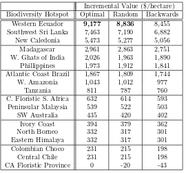
Table 1: Marginal value of land in biodiversity hotspots under different assumptions about search order.

Incremental Value ($/hectare) Biodiversity Hotspot Optimal Random Backwards

Western Ecuador 9,177 8,836 8,455

Southwest Sri Lanka 7,463 7,190 6,882

New Caledonia 5,473 5,277 5,056

Madagascar 2,961 2,863 2,751

W. Ghats of India 2,026 1,963 1,890

Phillippines 1,973 1,912 1,841

Atlantic Coast Brazil 1,867 1,809 1,744

W. Amazonia 1,043 1,012 977

Tanzania 811 787 760

C. Floristic S. Africa 632 614 593

Peninsular Malaysia 539 522 503

SW Australia 435 420 402

Ivory Coast 394 379 362

North Borneo 332 317 301

Eastern Himalaya 332 317 301

Colombian Choco 231 215 198

Central Chile 231 215 198

CA Floristic Province 0 -20 -43

search (in which leads are ordered in ascending probability of success). All parameter values are

held constant at the RS levels across these search experiments.2

Table 1 reports the expected marginal values from engaging in optimal, random, and backwards

search in each of the 18 biodiversity hotspots considered in SSR and RS. The optimal search column

reproduces the results reported in RS. The backwards search column simply reverses the order in

which research leads are searched. The random search column represents the expected marginal

value over all permutations of the search order.3

The table reveals, surprisingly, that search order has a small percentage impact on marginal

values. For example, searching in random order reduces the marginal value of a hectare in Western

Ecuador only 3.7%, from $9,177 to $8,836 (not $21 as in SSR), which is probably still sufficient

to justify private-sector conservation.4 _{In fact, even conducting maximally inefficient search (last}

2

We apply Equation 3 using the following parameters: R= 450e6,c= 485,r=.1,λ= 26.43,N= 74,640, and

pk= (1.2E−5)ekwhereekis the density of endemic species, per kilohectare, reported in RS.

3

In practice, this was calculated by 10,000 random permutations of the search order. The standard error of this approximation is<0.1% of the reported marginal value, for all figures in the Table.

4

column of the table) reduces marginal values only slightly.

What accounts for the negligible impact of information in this example? In Equation 2 we

separate the marginal value of a research lead into two additive components: aRevenue Component

and aCost Component. When using the RS parameters, the Revenue Component dominates; it is

responsible for about 93% of the marginal value of a lead. Importantly, it is clear by inspection that

theRevenue Component is independent of search order; it depends only on the termaN+1, which

is the probability of failure over the entire queue. On the other hand, theCost Component does

depend on search order. But because the empirical magnitude of theCost Component is relatively

small, the marginal value is not very sensitive to search order.5 _{Essentially, a lead has intrinsic value}

that relates to its ability to produce a success, regardless of the order in which it is searched. The

results of the experiment presented in Table 1 suggest that something other than efficient search

must account for the difference in estimates of conservation incentives. We next investigate in more

detail the true source of the discrepancy.

3

The source of the discrepancy

One of the key practical differences between the SSR and RS models is in the treatment of research

leads. SSR treat species as the relevant lead unit, and assume a constant success probability ¯pper

tested lead. In contrast, RS treat hectares as the relevant lead unit. We suspect the reason for this

divergence is to allow RS to embed heterogeneity of lead quality in a natural way. Since different

regions have different species densities, a given hectare in a heavily biodiverse region is more likely

to yield a success than a hectare in a less diverse region.

Given comparable parameterizations, this modeling change from species to land as research leads

should be inconsequential. The failure probability in hotspotkusingland areaas the unit of analysis

is: (1−pe¯ k)Nk/ek, where ek is the density of species, ¯pek is the probability of success per unit land

increases from $8,836 to $8,929).

5

area6 _{, and N}

k is the number of species in hotspot k. Following SSR, the failure probability in

hotspot kusing species as the unit of analysis is: (1−p¯)Nk_{. To see that these failure probabilities}

are close, consider the following approximation:

(1−pe¯ k)Nk/ek≈[(1−p¯)ek]Nk/ek= (1−p¯)Nk (4)

For this problem, the percentage difference between these two expressions is less than one

one-thousandth of a percent. Similarly, all other parameters of the species approach of SSR can be

constructed commensurately with the land approach of RS. However, care must be taken in the

parameterization in order to provide a fair comparison of conservation incentives. RS intentionally

selected their parameters to set the marginal value of the worst land to zero. This was intended to

illustrate their theoretical point that information could increase the value ofinfra-marginal leads.7

Below we show that this reparameterization is responsible for almost all of the difference in marginal

values.

To illuminate the source of the discrepancy between estimates, we adopt a strategy of sequentially

transforming the parameters of the SSR model until they are comparable to those in the RS model.

As we adjust each parameter in turn, we indicate by what multiplicative factor that adjustment

changes the calculated marginal values. It turns out that each parameter difference increases the

marginal value (wi in equation 6 below) estimates of RS relative to those of SSR. In comparing the

effect of parameter choices on marginal values, the order of parameter adjustment turns out to be

irrelevant, as it does not change the reported factors. This comparison reveals that most of the

difference in results between SSR and RS is explained simply by the use of incomparable parameter

values rather than by efficient search. After all parameters are made comparable, we introduce lead

heterogeneity. Finally, search efficiency accounts for the remaining (albeit small) difference between

results.

6

As specified by RS

7

Following SSR, the marginal value of a species (in pursuit of a single product) is

v= (¯pR−c)(1−p¯)N, (5)

where ¯pis the constant probability of success,Ris the revenue upon success,cis cost for each test,

andN is the total number of leads. Note that Equation 5 is a special case of the marginal value of

heterogeneous quality leads (Equation 2).8 _{Equation 5 has a simple interpretation. The marginal}

value of a species is the expected return in the event that the last species is sampled multiplied

by the probability of needing to test the last species. To convert marginal value per species to

marginal value per hectare, SSR employ a widely-accepted relationship between habitat area and

species abundance, known as the “species area curve”. In hotspotithe number of species conserved

with areaAi is: ni=αiAzi, whereαiandzare parameters. The increase in species with an increase

in area is the derivative, dni

dAi = zαiA

z−1 i =

zni

Ai. Denoting the density of species in hotspot i by

ei= n_Aii, the marginal contribution of area to species iszei. In the search for a single pharmaceutical

product, the marginal value of land is thenwi =vzei. If λsuch searches are conducted per year,

the marginal value of land in hotspotifor the purpose of bioprospecting in perpetuity is

wi = (¯pR−c)(1−p¯)Nzeiλδ (6)

where δ is a discounting term that gives the net present value over an infinite horizon (typically

δ= 1_r).9

We now compare thewivalues using the parameters in SSR and using the implied parameters in

RS to show that most of the difference between the two sets of results derives simply from parameter

choices.

• Number of species (N): Factor of 12.5. SSR assume a large pool of 250,000 plant species

across the globe and value those species (and the land that supports those species) within global

biodiversity hotspots. In the RS analysis, species outside the hotspots were not considered,

8

RS define the marginal value as the value ofdroppinga lead, while SSR define it as the value ofaddinga lead. To make Equation 5 a mathematically exact special case of Equation 2 therefore requires that Equation 2 be evaluated for thek+ 1 species with a total ofN+ 1 species. This discrepancy is extremely minor quantitatively.

9

SSR use the following parameters: ¯p = .000012, R= 450,000,000, c= 3600, N = 250,000,z = 0.25, ei ∈

[.00009, .00875],λ= 10.52,δ= 1

r = 10. Inserting these into equation 6 (wheree=.00875 for Ecuador) obtains the

leaving only 39,605 species. Reducing N to 39,605 increases marginal values by a factor of

(1−p¯)NRS

(1−p¯)NSSR = 12.5.

10

• Ecological model parameter (z): Factor of 4. SSR use the standard biogeography model

called the species-area curve. The concave curve depicts the number of species on a landscape

as a function of the area according to the equation ni =αiAzi. The parameter z determines

the degree of concavity. SSR assume z = 0.25. Given such a small value ofz, the marginal

contribution of new species by each additional hectare falls rapidly.

In contrast, RS do not explicitly specify a species-area curve. However, they assume that each

hectare in a region has a fixed probability of producing a success. In other words, they specify

a linear relationship between area and independent leads, z = 1. The value of the marginal

hectare will differ since SSR stipulate a concave species-area relationship while RS implicitly

use a linear relationship. Since z enters the marginal value calculation multiplicatively, the

change inz from 0.25 to 1.0 increases values by a factor of zRS

zSSR = 4.

• Number of tests per year (λ): Factor of 2.5. Both papers make the assumption that

multiple independent searches are conducted each year. SSR assume 10.52 tests per year, while

RS assume 26.43 test per year. Since searches are independent, the number of tests per year

simply scales up the value of a single search multiplicatively. The ratio of assumed number of

tests is 2.5, so changingλfrom 10.52 to 26.43 accounts for an increase by a factor of λRS

λSSR = 2.5

in values.

• Search cost (c): Factor of 2.5. The search cost in RS is $485 perkilohectare. The search

cost in SSR is $3,600 per species. To make the units comparable, we need to translate the

RS value to a cost perspecies. Searching all leads in RS would cost 74,640kha*$485/kha=$36

million. With a total of 39,605 species, this is a cost of $914 per species (the translation from

species to area is linear because RS assume z = 1, see above). This adjustment of c from

$3,600 to $914 yields a factor pR¯ −cRS

¯

pR−cSSR = 2.5 increase in marginal values.

10

• Probabilities (p¯): Factor of 1. The scientific model RS used to assign heterogeneous

probabilities ispRS

k = ¯pek whereekis the density of endemic species at sitek. By the

approxi-mation given in Equation 4 the failure probabilities in a region are numerically equivalent. The

SSR and RS probability models are therefore already comparably parameterized, requiring no

adjustment in ¯p.

• Other parameters. The remaining parameters are the same in the two models, so they

should not generate a discrepancy. We do note however that a minor coding error was made

by RS which leads to a practical difference in discounting between the two papers. Both

authors assume a discount rate of 0.10. SSR obtain the NPV over an infinite horizon with a

discounting term ofδ= 1_r = 10. While RS intend to conform, they use in their computer code a discount term of δ= 1+_rr = 11. This causes an additional (though minor and unintended) discrepancy of a factor of 1.1.

We thus find that no single parameter difference is responsible for the discrepancy. Taken together

these parameter adjustments result in an increase by a factor of 344 in the marginal value of a

hectare in each hotspot region. That is, simply by choosing comparable parameter values would, by

itself, increase the SSR marginal value in Western Ecuador from $21 to $7,095.

We have shown that simply reconciling the differences in parameters would account for most of the

difference between the bioprospecting value estimates in this literature. But an additional difference

between the two models is that RS assume that leads are of heterogeneous quality, while SSR assume

that leads are of homogeneous quality. The final step in a fair comparison then, is to introduce

heterogeneity in the quality of bioprospecting research leads. RS implement lead heterogeneity by

assuming that the cost to test all species in a kilohectare is constant but the number of species

per kilohectare, and thus the success probability, differs across regions. Alternatively, in keeping

with the SSR approach of regarding species as the leads, one could allow costs per species to vary

by region. Using this approach, comparable heterogeneous costs are calculated by ci = 485/ei.11

11

Numerically, the two approaches yield nearly identical marginal values for any given search order

(<<1% difference). Those regions with a low cost per unit success probability increase in marginal

value, while more expensive regions decrease.

Numerical results for the heterogenous case are exactly those already presented in Table 1. A

factor of about 1.2 for the highest marginal value results from the introduction of heterogeneity even

under random search, increasing the marginal values from $7,095 to $8,836. The essential result

on heterogeneity is that regions with a low cost per unit success probability have relatively high

marginal values — regardless of search order. The difference in models to which RS attribute the

discrepancy in results — search order — is responsible for the remaining difference: from $8,836 to

$9,177 (a final factor of only 1.04).

Efficient search guided by improved information, the theoretical contribution of RS, is responsible

only for 4% of the increased marginal value. Simply rectifying the (undefended) parameter differences

between the two models accounts for the remaining 96%, even under random search.

4

Defensible parameter estimates

We have shown that the significant wedge between an early estimate of bioprospecting-derived

marginal value ($21/ha) and a more recent estimate ($9,177/ha) cannot be attributed to efficient

search. Instead, the difference can be attributed simply to different parameter assumptions. This

result clearly raises the question: Which set of parameters is correct?

In fact, because these papers are intended to make primarily theoretical contributions, neither

set of authors rigorously defends the parameters chosen. SSR choose some parameters tomaximize

the marginal value estimates (e.g. ¯p), and others are based on “generous estimates” (e.g. R). A

reasonable interpretation of the SSR paper, then, is that $21/ha is perhaps anover-estimate of the

private-sector incentives.

RS, on the other hand, choose one parameter in order to force the marginal value of the 18th

hotspot to zero (c), and others are “based on those developed by Simpson et al. (1996)” (p.192).

interpretation of the RS paper is that $9,177 is perhaps anunder-estimate. Despite the overwhelming

attention that this literature has received by practitioners, it seems that the parameters used have

never been scrutinized carefully. In this section we present and defend plausible values of these

parameters.

We reviewed literature from economics, ethnobotany, ecology, genetics, and pharmacology to

marshall a set of defensible, citable values for each of the 7 parameters of the model in equation 6.

For each parameter, we identified several independent estimates from data in the published literature.

We report below the range of values found in this literature search. It is intended to capture the

full range of reasonable possibilities for each parameter. We then use these estimates to calculate

the marginal values of land in biodiversity hotspots. This procedure provides the first defensible

calculation of the true value of land in these biodiversity hotspots. The next subsection reviews

the literature for each of the parameters in equation 6. The subsequent subsection provides the

associated marginal value results, and relates those results to those obtained in previous literature.

4.1

Parameter estimates

We now briefly present the results of our search for defensible parameter values.

• Number of species (N): This is a measure of the total number of plant species on earth.

There is widespread agreement among taxonomists that the number of known plant species

is approximately 250,000 (Cronquist 1981; Farnsworth and Soejarto 1985). A more precise

interpretation would account for both known, and as-yet undiscovered species. Several

calcu-lations discussed in Fabricant and Farnsworth (2001) estimate this number to be approximately

500,000. We therefore use a range for N of 250,000 – 500,000.

• Ecological model parameter (z): This parameter concerns the shape of the relationship

between the total number of species on a landscape and the area of that landscape. The

parameter tends to vary depending on the types of ecological communities under investigation.

Kilburn (1966) reviews several such relationships, and finds that for plant species, they vary

z = 0.27. Keeley and Fotheringham (2003) estimate the parameter for plant species over

30 biogeographic regions. These estimates range from z = 0.17 to z = 0.35 with a mean of

z= 0.253. We use a range forz of 0.17–0.43.

• Number of tests per year (λ): Following SSR, we can back-out the number of tests per

year by acknowledging the probability of any given search being successful: λ = S

1−(1−p¯)N,

where S is the annual number of drugs approved per year that are derived from plants. The

number of drugs approved by the United States Food and Drug Administration per year from

1996-2003 has ranged from 17 to 53, with an average approval of 31 drugs per year. Estimates

of the percentage of total drug approvals that are naturally-derived also vary, but estimates

range from 14% (Proudfoot 2002), to 40% (Butler 2004), but are typically around 25%. For

the parameterS, we use a range of for S of 3–15. The values forλitself are then calculated

using the above equation and the parameter estimates for ¯pandN.

• Search cost (c): This parameter measures the actual cost of obtaining a plant tissue sample,

transporting it to a laboratory, and testing that sample for active enzymes. Because these tests

will be conducted to take advantage of economies of scale, the most significant portion of this

cost is in the laboratory testing. We contacted several molecular laboratories that specialize in

testing outsourced tissue samples to determine whether antibodies react in a particular way.

When executed in bulk, these tests cost between $4,000 and $18,000 per species tested (e.g.

Qualtek Molecular Laboratories, Santa Barbara, CA). We use a range forcof $4,000– $18,000.

• Discount rate (r): A special issue ofJournal of Environmental Economics and Management

(vol. 18, issue 2) was devoted to the empirical basis for discount rates. This series of articles

provided theoretical and empirical guiding principles for identifying the correct r. Based on

these articles, we use a range forrof 1%–10%. This range corresponds with the upper and lower

5% quantiles of estimates obtained in Weitzman’s solicitation of 2,160 economists’ opinions of

• Probabilities (p¯): The probability that any given plant will lead to a commercial drug

ranges considerably. The most optimistic estimate we encountered was 1-in-1,000 (Shackleton

2001). A more typical estimate is 1-in-10,000, and the most pessimistic value encountered was

1-in-40,000 (Onaga 2002). We therefore use a range for ¯pof .000025–.001.

• Net Revenue upon success (R): Upon discovery of a plant with promising chemical

proper-ties, a pharmaceutical firm must develop a commercially-viable drug and conduct three phases

of FDA-observed clinical trials to determine dosage, efficacy, and side-effects prior to actually

marketing that drug. Let ˜Rbe the present value of the revenue stream from selling the drug,

discounted to the time of drug approval. Now let ˜C be the cost of clinical trials required

to obtain approval to market a pharmaceutical product, also discounted to the time of drug

approval. Then net revenue at the time of drug approval is given by π= ˜R−C˜. The final

calculation of R requires discounting π back to the time of plant discovery. DiMasi et al.

(2003) estimate the mean time from the start of clinical trials to marketing approval is 90.3

months (7.5 years).

Grabowski and Vernon (2000) estimate the annual sales revenue, over a 20-year life of a drug,

for a sample of 110 new drugs. To obtain ˜R, we correct for inflation using the Consumer Price

Index and discount back to the time of drug approval. For example, withr=.10, the estimate

is ˜R=$1.2 billion. DiMasi et al. (1991) and DiMasi et al. (2003) estimate the expected cost

of transitioning through the three phases of FDA clinical trials. These papers estimate the

clinical trial cost per approved new drug, discounted to the time of drug approval, of ˜C=$104

million and ˜C=$467 million, respectively. We use the values given in Grabowski and Vernon

(2000) to calculate ˜R(which will depend on the discount rate). Our estimate of ˜Cfalls in the

range of $104 million–$467 million. The final calculation of R = R˜−C˜

(1+r)7.5, then, depends on the rate of discount, and on which estimate of ˜C is used. For example if r=.10 the implied

values ofRrange from $335 million–$513 million.

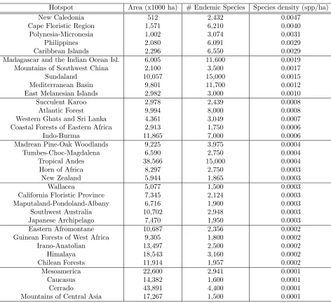
• Density of endemic species (ei): Both SSR and RS use data collected by Myers (1988)

of species in the 34 most biodiverse regions on earth (Myers et al. 2000; Conservation

Inter-national 2005). These calculations consider the present area covered with vegetation, rather

than the historical extent of vegetation in an area. Table 2 provides these updated hotspot

locations, number of endemic plant species, area of vegetation cover, and density of endemic

species.

The total number of known endemic species in these hotspots is 150,371. Note that the hotspots

in Table 2 are ordered according to the density of endemic species (and therefore, by marginal value;

see Figure 1 below).

Table 3 below summarizes the parameters used by Simpson et al. (1996), Rausser and Small

(2000), and the range of values used in this study. In general, our derived parameter ranges accord

with the values assumed by SSR.

4.2

New estimates of conservation value

For the 34 biodiversity hotspots shown in Table 2, we re-calculate the marginal value of land, using

equation 6, based on the full range of parameter estimates discussed above. Under the assumption

that the true parameter value is drawn from a uniform distribution over each range, and that these

draws are independent across parameters, we are able to calculate a mean and upper and lower 5%

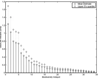
quantiles for the marginal value of each hotspot. These results are illustrated in Figure 1.12

Using the least favorable combinations of parameters, the marginal values are<0 because ¯pR < c;

such searches would never be undertaken, so the bioprospecting value is 0. Our mean estimate for the

most biodiverse region on earth is $1.23/ha, and 95% of the estimates of the conservation value of this

region are below $1.69. If the most favorable set of parameter values is used, the conservation value

for this hotspot could be as high as $300/ha.13 _{The value of less-dense hotspots is commensurately}

smaller.

12

We use 5 equally-spaced points over the stated range for each parameter, exhaustively enumerating all such combinations. We do not claim that the most reasonable subjective distribution is uniform. Rather, the assumption is intended to illustrate that it would require averyfavorable draw of parameters within the reasonable range to imply non-negligible values. A more plausible subjective distribution, which placed greater weight in the range center, would be less generous.

13

This number is obtained by applying equation 6 using the parameters:r= 0.01,p= 2.5E-5,c= 4000,z= 0.43,

Table 2: Number of endemic plant species, current vegetation area, and species density in 34 biodi-versity hotspots.

Hotspot Area (x1000 ha) # Endemic Species Species density (spp/ha)

New Caledonia 512 2,432 0.0047

Cape Floristic Region 1,571 6,210 0.0040

Polynesia-Micronesia 1,002 3,074 0.0031

Philippines 2,080 6,091 0.0029

Caribbean Islands 2,296 6,550 0.0029

Madagascar and the Indian Ocean Isl. 6,005 11,600 0.0019

Mountains of Southwest China 2,100 3,500 0.0017

Sundaland 10,057 15,000 0.0015

Mediterranean Basin 9,801 11,700 0.0012

East Melanesian Islands 2,982 3,000 0.0010

Succulent Karoo 2,978 2,439 0.0008

Atlantic Forest 9,994 8,000 0.0008

Western Ghats and Sri Lanka 4,361 3,049 0.0007

Coastal Forests of Eastern Africa 2,913 1,750 0.0006

Indo-Burma 11,865 7,000 0.0006

Madrean Pine-Oak Woodlands 9,225 3,975 0.0004

Tumbes-Choc-Magdalena 6,590 2,750 0.0004

Tropical Andes 38,566 15,000 0.0004

Horn of Africa 8,297 2,750 0.0003

New Zealand 5,944 1,865 0.0003

Wallacea 5,077 1,500 0.0003

California Floristic Province 7,345 2,124 0.0003

Maputaland-Pondoland-Albany 6,716 1,900 0.0003

Southwest Australia 10,702 2,948 0.0003

Japanese Archipelago 7,470 1,950 0.0003

Eastern Afromontane 10,687 2,356 0.0002

Guinean Forests of West Africa 9,305 1,800 0.0002

Irano-Anatolian 13,497 2,500 0.0002

Himalaya 18,543 3,160 0.0002

Chilean Forests 11,914 1,957 0.0002

Mesoamerica 22,600 2,941 0.0001

Caucasus 14,382 1,600 0.0001

Cerrado 43,891 4,400 0.0001

Mountains of Central Asia 17,267 1,500 0.0001

Table 3: Comparison of parameter values used in SSR, RS, and the current paper.

Parameter Simpson et al. (1996) Rausser and Small (2000) Range of new estimates

N 2.5E5 species 74,640 kha [2.5E5,5E5] species

z 0.25 1 [0.17,0.43]

λ 10.52 tests/yr. 26.43 tests/yr. [3,15.03] tests/yr.

c $3600 per species $485 per kha [$4000,$18000] per species

r 10% 10% [1%,10%]

p 1.2E-5 per species [1.1E-6, 1.1E-4] per kha [2.5E-5,1.0E-3] per species

R $4.5E8 $4.5E8 [$3.4E8,$2.2E9]

0 5 10 15 20 25 30 35 0

0.2 0.4 0.6 0.8 1 1.2 1.4 1.6 1.8

Biodiversity Hotspot

Value per Hectare ($/ha)

Mean Estimate Upper 5% quantile

Figure 1: Marginal value of land in biodiversity hotspots world-wide

Rather than assuming a constant probability of success for each species, we could adopt a model

in the spirit of Rausser and Small (2000), in which some species are known to be more likely to

yield a success than others. To explore this, we introduce heterogeneity by assuming there are 34

groups of species differentiated by research promise. Each species within a group has the same

success probability, but these probabilities differ between groups. The group sizes and probabilities

are engineered to have heterogeneity commensurate with that under the RS approach.14 _The

bio-prospector searches through these species in optimal order, exhausting the first group before moving

to the second. Species of each quality are present in all biodiversity regions, so that destruction of

habitat in any region destroys some members of each species group.

To explore the impact of ordered search under heterogeneity, we calculate the marginal value land

in each region. The important difference between regions is in the number of species driven extinct

14

These probabilities are engineered to give the same degree of heterogeneity as would obtain under the RS device of using land as research leads, with probabilities determined by species density. The success probability for species group

by destroying a set amount of habitat. Given this loss in species, the search must be conducted over

fewer research leads of all types, leading to a reduction in bioprospecting value — this reduction is

the marginal value of land. We calculate this marginal land value for the full range of defensible

parameter values presented earlier in this section. We find that the marginal value of the most

promising hotspots indeed increases under ordered search of heterogenous leads, to $14/ha (mean

estimate) and to $65/ha (upper 5% quantile estimate). While these numbers are significantly larger

in percentage terms than those derived under homogeneous leads, they unfortunately still lie below

what would likely be required for large scale private sector conservation via bioprospecting.

5

Conclusion

Can bioprospecting provide a sufficient incentive for private-sector biodiversity conservation?

Pre-vious work in this area has focused primarily on making conceptual contributions — perhaps at the

expense of empirically reliable estimates. Nevertheless, dramatically different answers have been

reported. The discrepancy has been attributed to efficient search guided by improved

informa-tion. In contrast, we have demonstrated that the strength of the bioprospecting incentive hinges

predominantly on the values chosen for several key parameters of the economic and biological

mod-els. Depending on the selected parameters, conservation incentives can be either trivially small or

quite large. We have attempted to resolve the outstanding question of bioprospecting conservation

incentives by providing a range of defensible estimates for each of the parameters in this model,

and recalculating the marginal value of land for bioprospecting. For most parameter combinations

within that range, marginal land values from bioprospecting are far too small to provide plausible

conservation incentives.

Our results are consistent with the empirical evidence of private-sector biodiversity protection,

where bioprospecting firms have been reluctant to invest in conservation for this purpose. Even

perhaps the most celebrated bioprospecting venture - between Merck & Co. and Costa Rica’s

National Biodiversity Institute (INBio) has resulted in a <$5 million investment by Merck; no

A very recent exception is the October, 2005 announcement that two products, an enzyme used in

the manufacturing of cotton and a fluorescent protein used as a chemical marker, were developed

from Costa Rican biodiversity. The products were developed by Diversa, an American biotechnology

company, who has entered a profit-sharing agreement with INBio. This was the first such success in

Costa Rica (INBio 2005).

Current private bioprospecting incentives are likely insufficient to induce significant investments

in biodiversity. However, future incentives could grow as more species suffer extinction (i.e. N is

reduced). For example if only those known endemic species in biodiversity hotspots were to survive

a mass extinction (leaving 150,371 species), our mean estimate would climb to $60/ha, and our

upper 5% estimate would climb to $268/ha.15 _{If both 3/4 of known species and all undiscovered}

species became extinct (leaving 62,500 species), the mean conservation value of the most biodiverse

land would rise to $700/ha and the upper 5% estimate would rise to $3,000/ha. — perhaps large

enough to offset the opportunity cost of development in some locations. Thus it might be that

bioprospecting could serve as a backstop preservation incentive after a catastrophic mass extinction.

While such an event may seem unlikely in the near term, this thought experiment raises some

interesting questions about the dynamics of land conversion, species loss, and associated

private-sector conservation incentives.

In summary, our results corroborate the pessimistic view of SSR that the bioprospecting

conser-vation incentive is insufficient to offset development. These results accord with the view that the

private-sector cannot, in general, be expected to efficiently provide public goods. To the extent that

biodiversity is a public good, other incentive mechanisms will be required for its protection.

References

Butler, M. (2004). The role of natural product chemistry in drug discovery. Journal of Natural Products 67(12), 2141–2153.

Conservation International (2005). Conservation international biodiversity hotspots.http://www. biodiversityhotspots.org/xp/Hotspots.

15

Cronquist, A. (1981). An Integrated System of Classification of Flowering Plants. New York: Columbia University Press.

Day-Rubenstein, K. and G. Frisvold (2001). Genetic prospecting and biodiversity development agreements.Land Use Policy 18, 205–219.

DiMasi, J., R. Hansen, and H. Grabowski (2003). The price of innovation: new estimates of drug development costs.Journal of Health Economics 22, 151–185.

DiMasi, J., R. Hansen, H. Grabowski, and L. Lasagna (1991). Cost of innovation in the pharma-ceutical industry.Journal of Health Economics 10, 107–142.

Fabricant, D. and N. Farnsworth (2001, March). The value of plants used in traditional medicine for drug discovery.Environmental Health Perspectives Supplements 109(S1), 69–75.

Farnsworth, N. and D. Soejarto (1985). Potential consequence of plant extinction in the united states on the current and future availability of prescription drugs. Economic Bontany 39(3), 231–240.

Firn, R. (2003). Bioprospecting – why is it so unrewarding. Biodiversity and Conservation 12, 207–216.

Grabowski, H. and J. Vernon (2000). The distribution of sales revenues from pharmaceutical innovation.Pharmacoeconomics 18(Suppl. 1), 21–32.

INBio (2005). Products generate resources for conservation. Press Release: http://www.inbio. ac.cr/en/noticias01.htm#interactive.

Kassar, I. and P. Lasserre (2004). Species preservation and biodiversity value: a real options approach.Journal of Environmental Economics and Management 48(2), 857–879.

Keeley, J. and C. Fotheringham (2003). Species-area relationships in Mediterranean-climate plant communities.Journal of Biogeography 30, 1629–1657.

Kilburn, P. (1966). Analysis of the species-area relation.Ecology 47(5), 831–843.

Koo, B. and B. Wright (1999). The role of biodiversity products as incentives for conserving biological diversity: some instructive examples. The Science of the Total Environment 240, 21–30.

Myers, N. (1988). Threatened biotas: hot spots in tropical forests.Environmentalist 10(3), 187– 208.

Myers, N. (1990). The biodiversity challenge: expanded hot-spots analysis. Environmental-ist 10(4), 243–256.

Myers, N., R. Mittermeier, C. Mittermeier, G. da Fonseca, and J. Kent (2000). Biodiversity hotspots for conservation priorities.Nature 403, 853–858.

Nigh, R. (2002). Maya medicine in the biological gaze.Current Anthropology 43(3), 451–477. Onaga (2002, May). Cashing on in nature’s pharmacy.EMBO Reports.

Polasky, S. and A. Solow (1995). On the value of a collection of species.Journal of Environmental Economics and Management 29(3), 298–303.

Polasky, S., A. Solow, and J. Broadus (1993). Searching for uncertain benefits and the conservation of biological diversity.Environmental and Resource Economics 3, 171–181.

Preston, F. (1960). Time and space and the variation of species.Ecology 41, 611–627.

Proudfoot, J. (2002). Drugs, leads, and drug-likeness: An analysis of some recently launched drugs.Bioorganic and Medicinal Chemistry Letters 12, 1647–1650.

Rausser, G. and A. Small (2000). Valuing research leads: bioprospecting and the conservation of genetic resources.Journal of Political Economy 108(1), 173–206.

Simpson, D., R. Sedjo, and J. Reid (1996). Valuing biodiversity for use in pharmaceutical research.

Journal of Political Economy 104(1), 163–185.

South Asian Network for Development and Environmental Economics (2003, February). Sandee newsletter #6.