Graphical methods for the analysis of data

Graphical methods for the analysis of data.

Available from Sheffield Hallam University Research Archive (SHURA) at: http://shura.shu.ac.uk/19819/

This document is the author deposited version. You are advised to consult the publisher's version if you wish to cite from it.

Published version

HOLMES, David I. (1972). Graphical methods for the analysis of data. Masters, Sheffield Hallam University (United Kingdom)..

Copyright and re-use policy

SHEFFIELD CITY POLYTECHNIC LIBRARY

POND STREET

SHEFFIELD SI 1WB _{$ 1 $}

Sheffield City Polytechnic Eric Mensforth Library

REFERENCE ONLY

This book must not be taken from the Library

P L/26

GRAPHICAL METHODS FOR THE ANALYSIS OF DATA

t o

DAVID I. HOLMES B.Sc. M.I.S. F.S.S.

A thesis submitted to the Council For National Academic Awards for the degree of Master of Philosophy,

I

ACKNOWLEDGEMENTS

I v/ish to express my sincere appreciation to Dr. W.G. Gilchrist and Dr. D.S. Houghton for the guidance received during this research programme.

I should also like to express my thanks to the following:

- W. Jessop for his guidance in the formulation of the computer programs.

- The M.R.C. Unit of Middlewood Hospital, Sheffield (Director: Professor F.A. Jenner) and the

Department of Chemistry and Biology, Sheffield Polytechnic, for the use of their data.

PREFACE

The content of this thesis is divided into two parts. Part I consists of a review of graphical methods in data analysis, whilst Part II presents a graphical procedure for identifying growth

Page 1 5 10 16 24 36 40 43 48 59 79 88 89 92 94 96 100 CONTENTS

Part I. A Review of Graphical Methods in Data Analysis

The history of graphics. Probability plotting.

Graphical methods for discrete data.

Graphical methods for data from uniresponse experiments.

Graphical methods for multivariate data. Graphical methods for growth curves.

Part II. A Graphical Identification Procedure for Growth Curves

Foundation of the identification procedure. The least squares fitting process.

Plots for model identification. Choosing the "pf! terms.

Results and conclusions. Areas for further research.

References

Appendices

Determination of the g(r,s) terms in the least scmares fit.

The inverse of the truncated [g(r >s)j matrix.

no

Some results concerning the coefficients aj (j*0,l,...4) for simple modified exponential data.

Error analysis for the asymptotic values of 0 . , A . o v • and o • ._{m m ’ m m * m m Hm m}

PART I

A REVIEW OF GRAPHICAL METHODS

IN DATA ANALYSIS

CHAPTER 1

THE HISTORY OF GRAPHICS

Graphical presentation of statistics was intro­ duced at the end of the eighteenth century. There is some doubt as to whether the ’’inventor” was William Playfair (1759 - 1823) or A.F.W. Crome (1753 - 1833). Playfair’s works on general descriptive economics were illustrated i^ith some extremely good graphs, histograms and pie diagrams, whilst Crome devised charts to des­ cribe geographical data of European states, chiefly population figures and areas. Crome justified the use of his geometrical representation as follows:

’’The proportions of the different sizes can how­ ever be more easily seen and grasped if they are brought before the eye in the form of a drawing, because the imagination is thus stimulated, than if these merely appeared in the form of numbers, especially when these consist of many digits as is often the case with areas of states...” (Crome {10} 1785)

A detailed investigation of the work of Crome and Playfair has been undertaken by Royston {29}.

Applied Mathematics and it was only natural that he should extend this approach to Statistics.

In 1915 Fisher {14} used 3-dimensional geometry to describe a mean, a standard deviation, and Student's ratio, and in 1925 wrote:

"The preliminary examination of most data is facili­ tated by the use of diagrams. Diagrams prove nothing, but bring outstanding features readily to the eye; they are therefore no substitute for such critical tests as may be applied to the data, but are valuable in suggesting

such tests, and in explaining the conclusions founded upon them.1’ (Fisher {15})

In 1949 Hosteller and Tukey {25}, in an article on the use of binomial probability paper, drew attention to the advantages of employing graphical methods to analyse data.

"The speed of graphical processes, and the advan­ tages of visual presentation in pointing out facts or clues which might otherwise be overlooked, make graphical analysis very valuable." (Mosteller and Tukey {25})

In the early 1960’s, possibly motivated by articles by Tukey {31,32,33} on data analysis, statisticians began detailed investigations into the use of relatively un­ sophisticated procedures for extracting information from a body of data, in particular the use of graphical pro­ cedures. Tukey wrote:

"Procedures of diagnosis, and procedures to extract indications rather than conclusions, will have to play a large part in the future of data analysis. Graphical

Wilk and GTlanadesikan, who were to play leading roles in the development of graphical procedures for the analysis of experimental data, also commented on the need for graphics and informal data analytic pro­ cedures :

"If statistical methods are to be relevant to the analysis of data, then a major concern of theoretical statistics will have to be the provision of methods which are useful tools for ’learning from’ data and for bringing out the latent information in data. There are greater possibilities of gaining insight into data

through, the use of an informal method, like probability plotting, than through the use of a formal technique like a test of significance." (Gnanadesikan {17})

Tukey was particularly concerned that graphical procedures should involve straight line ccmfigurations as often as possible.

"Graphs are most effective ... when reference

situations produce straight lines." (Tukey and Wilk {33}) When comparing data with a fitted curve he advo­ cated improving the histogram "by employing:, instead, a hanging rootogram (see Figure 1) in which the blocks are attached to the fitted curve (not the base line) and the eye merely has to check on the ’straightness" of t h e c > f rootogram.

•CE fAQ

! — Half-norm al plot of a 2s experim ent. D ots and solid lino-31 contrasts. Crosses i dashed lino-21 sm allest contrasts.

1

F i q o / S E I*.

F \ q o R . £ _I

RooTo«i^flM

Batch

Sample s , s 21 S sa2 3 s s 2

4 S %

5 s, s2

6 s , s 2

7 SA

8 s , s £

15-0 + +

^ 15-6- a ‘o

«3 + « + + e

15-4 + e + e

V c

4-£ 15 2 • ©

§>

4-150 4" • e + • + ©

1 © ©

£ 14-8 ©4- +■

14-6 • +

Result of ana (t/5 is by ®

FiquflF

3

£(Z(Ztofl$ Op

flhJ^jLVStS

d

o

'43_o

d

<h c.d.f.y.

d o 4 ^ c3 r —i s£ d O o

Q u antiles

FltjoftE a,

Tu.uST/ZfiTtod

p_ p

by Tukey:

"Computer-drawn graphs .... are going to be the data analyst’s greatest single resource." (Tukey {32}), and is now widely advocated:

"The graphic aspect of the computer can rapidly convey the results of a computation to the man in a form that can be quickly perceived i.e. through the man's visual senses." (Ball and Hall {3}).

"The thorough graphical analysis of residuals as a routine is feasible only with a suitable com­ puter graphical output device." (Cox and Snell {9})

CHAPTER 2

PROBABILITY PLOTTING

(a) Uses

It is often useful in data analysis to treat a body of data as though it were an unstructured array. A valuable representation of such data is provided by

the empirical cumulative distribution function

(e.Cod.f.) i.e. a plot of the i ’th ordered value as ordinate against i - \ _{as abscissa (i = 1, .. .. n) .}

n

Wilk and Gnanadesikan {39} have discussed in detail the advantages of the e.c.d.f., in particular its effectiveness as an indicator of peculiarities e.g. asymmetry. They devised two basic kinds of plots for situations where either (i) two e.c.d.f.’s are to be compared, (ii) an e.c.d.f., is to be compared with a theoretical c.d.f., or (iii) two theoretical c.d.f.fs are to be compared. Their plotting procedures may be described with the aid of Figure 2.

Corresponding to any ordinate value p there are two quantile values (p) and (p) . A scatter plot °f against qx (p) for various p, they label a

"quantile versus quantile" (Q~Q) plot. Similarly, corresponding to any abscissa value q, there are two c.d.f., values px (qd and py(q,). A "percent versus percent" (P-P) plot is just a scatter olot of p (a)

y

against pv (q) for various a.

with slope unity, pointed towards the origin. Q-Q plots are especially sensitive to discrepancies in the tails of the distributions, whilst P-P plots are sensitive to discrepancies in the middles of the distributions.

Wilk and Gnanadesikan mentioned that extensions and hybrids of the P-P and Q-Q plots could be used but suggested that more investigation was required for the applications of these techniques.

Probability plots act as useful, informal aids to inference in data analysis. The essence of such plots is to plot the n ordered ’’sample” values against some representative values from a presumed standard distribution. • There are essentially two choices of representative

values:-(i) corresponding quantiles of the reference distribution such as i - 1 _{*- or ----=-}i

n n + 1

(i = 1 n) , plotted on the appropriate probability paper,

(ii) expected values of the standard order stat­ istics from the reference distribution .

Under certain null statistical conditions a linear configuration is obtained, passing through the origin. The presence of real effects in a designed experiment » the existence of distributional peculiarities, of

Probability plots of the individual residuals in regre­ ssion studies are informative and sensitive tools. The graphical analysis of residuals will be surveyed in Chapter 5. Probability plots may also be applied to analysis of variance situations and a detailed study of this particular application is made in Chapters 4 and 5.

(b) Choice of Plotting Positions

The choice of plotting positions on probability paper has been investigated by Chernoff and Lieberman {6,7} and Kimball {22}. Chernoff and Lieberman consi­ dered the problem of graphically estimating the mean, y, and standard deviation, a, of a normal population on

the basis of a sample. If Xj , x2 , .... xn denote the ordered sample values and P i P 2 > • • • • Pn ‘t^ie appropriate values on the probability scale, then the problem was, essentially, what values of theP ls yield good estima­ tes, y and 6? In order to translate the process of visually fitting a straight line to the set of plotted points into an analytical process, Chernoff and Lieberman proposed the assumption that the visually fitted line is a very good approximation to the line that would be obtained by minimizing the sum of squares of the devia­ tions (in the x direction) from the line. This process yielded sampling variances of the resulting analytical estimates of the parameters y and a _.

Their criterion for judging the optimal character of a plotting method was _{the resulting magnitude of}

p^ (i = 1, ..., n) , for various n, which minimized the variance of an unbiased estimate of a. They also showed that a biased estimate of a with minimum mean square deviation could be found, and the plotting positions for this estimate were given. They conclu­ ded that the optimum choice of the p ’s depended upon whether an unbiased estimate was necessary or whether

a biased estimate could be tolerated.

Kimball extended the work of Chernoff and Lieber­ man by pointing out that probability paper was not used merely to estimate parameters. There were two other purposes served in using probability paper,

namely, as a test as to whether or not the sample data indicated that the population was of the prescribed type, and for graphical extrapolation at one of the extremes, the purpose most commonly served when plott­ ing data from an extreme-value population.

both normal and extreme-value populations a conven­ tion attributed to Blom {5}, p. = (i - j) ,

(n + 3)

would be satisfactory and simple to use for all three objectives for using probability paper. This conven­ tion carried an estimate of the scale parameter with low mean square deviation.

Kimball emphasised that there was need for caution in relying upon any single formula and that, parti­

cularly for extrapolation for an extreme-value popula­ tion, it would be well to supplement the plot using points determined from other conventions.

Blomfs convention never seems to be used in prac­ tice. Text books tend to use plotting conventions based on order statistics, namely p. = i or

n + 1

p. = i - I , between which there is no difference

1 n

CHAPTER 3

GRAPHICAL METHODS FOR DISCRETE DATA

(a) Binomial-Like Counts

Dubey {12} proposed a graphical test to determine whether certain experimental data could be described satisfactorily by a binomial distribution,, If, in the standard binomial notation,

p(i) = Pr {X = i) = H n e1 Cl - e)n_i (i = 0,1,2, .... n),

then

p(i+l) = - 6 + (n+l)6 . 1... ... (3.1) p(i) (i-e) (i-e) (i+i)

Hence, plotting p (i+1) against 1 should give a

p{i) i+l

straight line with slope (n+1)6 and intercept - 6 ,

1-0 1-9

This method requires an estimate of the unknown parameter 0 in order to calculate p(i). In a later paper Ord {26} noted the relationship i p(i) =

p(i-l)

(n+l) 0 - 0 o i (i = 1,2, .... n) and sugges-1-0 1-0

ted that, using the assumption f^a p(i), where the f^

denote frequencies for the cases X = i (i = 0,1,2, .... n) , a plot could be made of i f^ against i. This should

7 l-l

give a straight line with slope - 0 and intercept

(n+l)0 . 1”G

Gart {16} suggested the simpler relationship

_______i p(i)_________ = 9... ... (3.2) (n-i+l)p(i-1) + i p(i)

and showed how a plotting technique derived from (3.2) is related to estimators and statistical tests of full or nearly full efficiency. Using Ord's assumption that f. ap(i) we have a set of estimators

- i f.{( n - i + l ) f . + i ^i>~1 (i = 1,2,3 n) .

A logical estimator of 0 is the weighted mean of the 0., namely 0 = ?^i0i . If w. = (n-i+l)f. 1 + i f .

Ew. 1 1

^ Eif 1

then -0 ■= i__ i = _i which is, of course, the best esti- nEff n_{i l}

A

mator. If the 0^ ’ s are plotted against i they should cluster around the horizontal straight line with

ordi-A

nate 0.

Gart derived a normal deviate test to test whether

A A

any particular 0^ deviated significantly from 0. He pointed out that this test did not involve a specific alternative to the binomial distribution and suggested, as a reasonable alternative, the bet?-binomial distri­ bution ,

p(i) = Pr{X=i} = (n\ _{3(a+i,0+n-i) (i =0,1, .... n)}

^i) _BfcTFl

where a and $ are positive constants. Manipulating as in (3.2) we obtain

i p (i)__________ = q-1 + i (n-i+l)p(i-1)+ip(i) a+3+n-l a+0+n-l

analysis, this is equivalent to 0^ = C + Di where C and D are certain constants. If the data deviated from the binomial in the direction of the

beta-A

binomial, the plot of 9^ against i would be linear with positive slope. The hypothesis that the data

is binomial as opposed to beta-binomial can be formu­ lated as H : D = O; H1 :0<D<(n-l) ^. Gart showed that a test based on D, the weighted least squares

?

estimate of D, is equivalent to the homogeneity y~ test. This is the asymptotically locally optimal test for the binomial against the general alterna­ tive of 0 being itself a random variable. Hence the "best” test of the binomial can be related to a simple and informative graph. The graph may also be used to estimate the parameters of the beta-binomial distri­ bution ;

(b) Poisson-Like Counts

Using his ideas set out in the previous section, Dubey proposed a graphical test to determine whether certain experimental data could be described satis­ factorily by a Poisson distribution. If, in the stan­ dard Poisson notation,

p (i) = Pr{X= i} = e~X A1 (i = 0,1,2.... ) (A>0) , i I

then

p (i) = 1 + 1 i pti^lj X* X

Hence, plotting p(i) against i should give a straight p U +l)

line with slope 1_ and intercept 1. Dubey commented

that the method required an estimate of the unknown parameter A in order to calculate p (i) , and Ord later derived an alternative relationship, namely

ip (i) = A (1 = 1,2,3,....), from which, using his P (i-l)

i assumption f-ap(i), it follows that a plot of i

1-1 against i should give a horizontal straight line with­ er dinate A .

In a manner similar to his work on binomial- like counts, Gart showed how Ord's plot could be related to estimators and statistical tests. A logi­ cal estimator of A is the weighted mean of the esti-

/s • r Z W A

mators A . = i i.e. A = i i i . I f w . =f. n then

1 _± 1

A

A takes the value T which is the best estimator.

Gart’s normal deviate test to test whether any

parti-A /V

cular A^ deviated significantly from A did not, as in the binomial case, involve a specific alternative to the Poisson distribution. He suggested, as a reasonable alternative, the negative binomial distri­ bution p(i) = Pr{X=i} = ^ + _{r 1}

(i = 0,1,2, . . . .) (m,r>0).

In a similar manner to the derivation of (3.1), Dubey has shown that

P (i) =

fl

f

and that a plot of p(i) against 1^ should give a

P(i + iy i

This however5 while providing a useful

test in itself, was not directly compatible with plotting techniques used for the Poisson distribu­ tion. Gart rectified the situation by noting that Ord had proved the result

either Poisson or negative binomial. In the latter

D are certain constants. Thus, if the data is con­ sistent with the negative binomial, the plot of A. against i would be linear with positive slope.

A test of the deviation of the data from the Poisson assumption in the direction of the negative binomial alternative can be formulated as H : D = 0 : 0<D<1. Gart showed that a test based on D, the weighted least squares estimate of D, is equivalent

to the asymptotically locally optimal test of the Poisson distribution against the negative binomial alternative. Hence the "best” test of the Poisson distribution can be related to the graph.

The logarithmic series distribution of Fisher i £

which enabled a plot of i against i to indicate

^ *

case this is equivalent to L s C + D.l where C and

o

is defined by p(i) {X = i.} = a61 (i = 1,2,3,....1

configuration with positive slope. This log series plot could possibly be confused with the negative binomial plot, a fact which motivated Gart to investi­ gate other plotting relationships, notably

i p(i) = 0 (i = 2,3....). The individual (i-l)p(i-l)

i f *

estimators of 0 are 0. = i and the 0.fs

1

TZZTt

should cluster around a horizontal straight line when the data fits the log-series model.

(c) General

Grimm {20} showed that the types of some dis­ crete distributions could be readily discerned by plotting data on Poisson cumulative probability paper. Transparent stencils were used to quickly recognize typical curves and to estimate their para­ meters. The class of compound and generalized

Poisson distributions is represented by curves in­ clined to the right, while the (positive) binomial is versed to the left.

Ord plotted i p(i) against i for several dis- p(i-l)

crete distributions. In the case of the hypergeo­ metric, beta-binomial and beta-Pascal distributions, curves were obtained. Graphs are most effective for identification purposes when linear plots are produced so Gart's work on the derivation of straight line configurations, e.g. beta-binomial distribution, is a welcome extension of Ordfs technique.

-CHAPTER 4~

GRAPHICAL METHODS FOR DATA FROM

UNIRE SPON SB EXPE RIMENTS

(a) Plots of Raw Data

In 1956 Pearson {27}, concerned at the lack of evidence of statisticians ’’geometrically examining the pattern of their data” before analysing it arith­ metically, described simple ways for graphically in­ specting data in analysis of variance situations. Figure 3 shows the data from an experiment with eight batches of fertilizer, two independent samples (S^, S2 ) being drawn from each batch, each sample then

being divided into two sub-samples, the first ana­ lysed by method A, the second by method R. The var­ iable measured was ’’percentage of potash”. Inspec­ tion of the plot indicates that with the exception of Batch 3 the difference between the two results for a given batch, using the same method of analysis

(either A or R) is small. The determinations by methods A and R, however, differ considerably. Sub­ sequent arithmetical analysis confirmed these find­ ings .

(b) Probability Plots

Half-normal probability paper is prepared by deleting the probability scale P, for P < 50%, on normal probability paper and replacing each P value by P' = 2P - 100 , for P > 50%0 The absolute value of the i'th smallest contrast is plotted as abscissa, against P* = (i ~ I) (i = l,2,....n) where n is the

n

number of contrasts obtained from the experiment. If there are no real effects then the plotted points follow a straight line with positive slope, passing through the origin. An estimate of the standard error of the contrasts may be obtained from that contrast for which P ! is most nearly 68.3%. A par­ ticular treatment factor or combination of factors is judged to have a real effect if the corresponding contrast appears to be "too large" relative to the other contrasts in the configuration of the half­ normal plot. The plot may then be revised by omitt­

ing these contrasts and obtaining a new estimate of the standard error of the remaining contrasts as before (see Figure 4).

In his paper Daniel included some remarks of Tukey's on half-normal plotting. Tukey had prefered a grid that used the logs of the absolute values of the contrasts since the corresponding expansion of the scale for smaller contrasts would be useful. Tukey also suggested inclining the contrast axis at 135° to the positive horizontal in order to bring the expected position of the plot for experiments

-with no real effects to a horizontal straight line. This would be useful in the sense of easier visual identification of real effects but the plot would lose its inherent simplicity.

Daniel added that half-normal plotting could - lead to (i) overestimation of the standard error of

the contrasts, (ii) the omission of a number of real effects, (iii) faulty identification of real effects and (iv) possible non-detection of "defective1* con­ trasts due to their being masked by real effects. Rirnhaum{4) commented that Daniel's graphical method had the advantage that it gained, from the data being analysed, a degree of confirmation for the under­

lying assumptions used in analysis of factorial experiments, namely, that the contrasts are indepen­ dent and normally distributed with common variance and that certain high-order interactions are zero. Birnbaum was interested in an alternative to the stan­ dard assumptions and developed his own inference procedure for detecting real effects. This could be carried out within Daniel's graphical procedure.

In a series of papers (17,18,34-40} Wilk and Gri&nadesikan developed procedures to supplement the analysis of variance table by helping in the follo­ wing respects: (i) allowing the data themselves to provide guidance in developing an error term, (ill giving an easily grasped summary with a focus of attention on interesting features such as real

assumptions. A useful objective analysis of variance is the ioint relative assessment of com­ parable quantities e.f. a collection, of mean squares or contrasts in a 2n experiment. Wilk and Gnnna- desikan labelled procedures which involve the sim­ ultaneous comparison of comparable quantities through the use of a statistical measure or stan­ dard , "internal comparisons'' procedures. They

pointed out that Daniel's procedure provided graphi­ cal internal comparisons of a set of single-degree- of-freedom. contrasts in uniresponse experiments. The graphical nature of the method facilitated the gaining of insight concerning the structure of the data although in this respect they thought it

better to include both half and full-normal riots. Wilk and Gnanadesxkan devised graphical inter­ nal comparisons methods for analysing experimental datao Their work may be summarized with the aid of the following

classificationsr-RESPONSE STRUCTURE

Decomposition of _c--- TT . _Univariate . , _Multivariate, Treatment Structure

All 1 _{d.f. I} XV

All v d.f. IT V

Mixed d.f. Ill VI

Experiments of the type denoted by Cell II are those where the treatment structure is to be analysed in terms of ecjual (>1) degrees of free- dom decompositions e.g.. the comparison of all

main effects in a three-level factorial experiment. Wilk and Gnanadesikan devised a gamma probability plotting procedure for such data where the n ord­ ered squared contrasts are pi otted against approp­ riate cjuantiles of the standard gamma distribu­

tion (scale parameter, X 3 = 1) with shape parameter,

irj s e<jual to i Vo

What is involved in obtaining such a plot is

{b-} (i = l f2„,«.n)* defined usually as b. =_{1 • 1} 1 - I , and to determine quantiles x. such that

Wilk, Gnanndesikan and Huyett {35} provided tables listing x. for values of ^ and b^. The i’th

ordered squared contrast is then plotted against

x. on ordinary linear by linear graph paper. Under a null hypothesis of no real effects the squared contrasts may, as a reasonable approximation, be considered as a random sample from a gamma distri­ bution with scale parameter X unknown. It can easily be showsi that, under such an hypothesis, a straight-line configuration should be obtained with intercent 0 and slope 1_. The contrasts

to calculate an increasing sequence of proportions

n

x

o

associated with real effects will appear as "too large” deviations from the straight line pattern

(see Figure 5).

Gamma probability plots also serve as important tools for detecting other "peculiarities” in the data such as distortions due to "maverick” observa­ tions and bad non-normality of the original data. The gamma distribution has been considered as a model in life-test problems and an evaluation of

this assumption, or of an assumption of exponen- tiality, is possible through a gamma plot of ord­ ered failure times.

Wilk and Gnanadesikan derived a graphical inter­ nal comparisons procedure {40} for Cell III of the table i.e. for experiments where the analysis of variance mean squares may have differing degrees of freedom. The procedure consisted of plotting the ordered mean squares against representative values defined as expected values of appropriately condi­ tioned order statistics of standardized mean squares. If the ordered values of the mean squares are den­

oted by with corresponding

degrees of freedom v1,V2 «....v^ respectively, then

the standardized mean squares are such that the ifth ordered standardized mean square, Vh, comes

y ^

from a A distribution (i = 1,2,...K). One

of the "null” assumptions is that the i'th mean

-W eight o f cork b orin g (incent,grams)

30 ^ 40 so 60 -70 80 90 iqq

1 • i '—i— • 0 -hs

2 • 0 A +

3 4 5 C 7

• 4 4 O 8 44 4 O -»

4 4 8

.+

Orientation : N 0 E © S + W A 8 4 4 06

9 4 4 0 6 10 + • o < 11 A • 0 +

12 c 2 +

13 © AO +

oJ 14 ILl at 15 H 16 o 17

A O ©+

+ A 0 A

A # • • + o

0 +

tc 16 A + CO

to 19 • A + o § 20 4 O

2 21 -fO AO 22 _{$ 8}

23 • < O +

24 OCA +

25 A. ♦ ? 26 • + A 0 27 • + 0 A

26 A

— - I.. Ill „ 1 ■ 1____ O 0 4

s M B oR.E HEAT'S _CsF

o fi C o ft tc ~ T % E £ S

i Ii i ii ! I I | I J s j !

FiquRG. 7

tot_o 1.381.21

1.04 0.86 0.69 0.52 0.35 0.17

0 lno cl L©

© ExS

G

SxTOC

J L

TOC x E

B(10)x 10

137

114

2 0.91

I

w $ 0 6 9

0 4 6

0 2 3

0 0.78 1.56 2.34 3.12 3.90 4.68 5.46 6.24

•r E

*( • A

o1 ■ . C. • •

B'

• H <

r«c;o£e b

SR. ftLl'Z.E.J) _toflflSlUT/

pL.oT

0 9 2 1.38 1.04 OUANTILES

Ft s u & e 5

P/-oT

square is distributed (in the absence of real effects')

2 2

as ^ v~i where a2 is a presumed common error var- vi

iance. It follows that E{S^ | v^v2 ,... .v^} =

a2E{V^|Vj,v2,....v^} and hence if 0^ = (constant)

E{V.I Vi,v2j•••.vj then a plot of S. against 6._{1 l \ 3. 1}

(i = 1....K) would be expected to yield a linear configuration, with a slope which depends on a2 , when the mean squares do indeed conform to null

assumptions. Wilk and Gnanadesikan developed com­ puter programs for calculating the 0^. With real experimental effects, the associated mean squares would tend to appear as departures from the linear configuration (see Figure 6).

(c) Transformations

An aspect of great importance in data analysis is the transformation of variables. Data from a factorial experiment with large interactions may sometimes be described without interactions if it is first transformed. Kruskal {23} developed a graphical procedure where the _{data itself indica­}

ted the monotone transformation which made the inter­ actions smallest. In the general linear model a set of observations Y^ (i = l,....n) are such that it is supposed jr^ _{= E{Y^} =} Z _{^ij^j where the}

g.. are known numbers and 3. are unknown parameters._{^-3 3}

When this model fails to fit the data it may be

assumed instead that some appropriate transformation

-Z. = f(Y^) satisfies the structural relationship,

as a measure of disparity betx^een the numbers and the numbers z^. Minimising S(f,B) over $

Kruskal labelled the resulting quantity S(f), the "metric stress" of the numbers Z^. The "best" mono­ tone function, f, is defined to be the one which minimizes S(f). f is an estimate of the true under­

lying function f, and is labelled the "minimum • stress function". The shape of this function, when plotted, indicates the appropriate transformation.

In Figure 7 the minimum stress function is shown as a jagged curve and is compared x^ith a logarithmic function, the smooth curve. The asterisks show

3* + Y- + 6, against Y. _{1 1 k 11k} x^here Y. _11k denotes the

data and Z.., = f(Y..,) is such that E(Z..,} =_{11 K 11 K 13} Zi = = w^ere t^ie function f must be

i

determined. Kruskal used the quantity

CHAPTER 5.

GRAPHICAL METHODS FOR MULTIVARIATE DATA

(a) Plots of Raw Data

In a similar manner to his work on univariate data described in the previous chapter, Pearson {27} emphasized the importance of a preliminary graphical study of data when several variables are used.

Figure 8 illustrates such a study where the thick­ ness of bark deposit on cork trees is measured for 4- tree orientations, North, -South, East and Nest.

Visual examination of the data indicates that, besides the very noticeable between-tree differences, there are differences in pattern associated with the

ordering of the trees. It is therefore doubtful whether, without further sub-division, the data would be sufficiently homogeneous to justify any conclusions being drawn using multivariate normal theory.

(b) Probability Plots

If "knowledge were available to permit equal wei ght- ing to the responses, Will: and Gnanadesikan suggested that an informal study of the data could be made by conducting a half-normal plot on the absolute values of a variable defined as the sum of the contrasts for each of the responses corresponding to a particular effect.

Roy {28} suggested a way of looking at the multi­ response problem as a sequence of uniresponse pro­

blems. If, for example, response P., is more important than response D^s then the bivariate assessments of

and should be thought of as the sequence of assessments: (i) with respect to marginally; (ii) with respect to conditional on . Wilk and

Gnanadesikan extended this idea to a graphical pro­ cedure involving two half-normal plots, both necessary for a study of the data. One plot used the absolute values of the contrasts for response only, whilst the other used the contrasts for the ’'conditional response MJ)? given These contrasts are obtained essentially from an analysis of covariance of with response as a covariable.

Wilk and Gnanadesikan devised a gamma probability plotting procedure for situations where there is no meaningful basis for ordering the responses. If p

yi = (yil> yi2’ _{7ip)• The N x p matrix o}

observations is then given by

Ai\

2

Y _r'

v— y

For uniresponse situations, the conventional esti­ mates of the overall mean, main effects and inter­ actions may be viewed as being essentially given by an appropriately chosen orthogonal transformation of the observations. If R is the appropriately

chosen N x N orthogonal matrix, then, for the multi­ response situation, application of the same trans­ formation R to Y yields

^ j = R Y where n/ = (m^n^s. . . .m^)

is times the overall mean vector and X ={x • •}₃

(i = 1, . . ,.N-l; j = 1,.. . op). The rows of X are ”single-degree-of-freedom contrast vectors” e.g. the i’th row, denoted by x/ = (x..,, x.0....x. _{5 7 _ i ^ i l ? i 2 i p 7 s} has

as elements the contrasts for each of the p responses corresponding to the i ’th treatment effect.

Will? and Gnanadesikan introduced a measure of ”size” to go with each of the contrast vectors. For the contrast vector x^„ they associated the measure

of size d. , defined by d- = x_{i i _} f _{A x. where .A is an}

j l — 1 —

as the ’’compounding” matrix. If A was chosen to be the identity matrix then would be the sum of sauares of the elements of x^. Under a null hypo­ thesis of no real effects the ’’distances” d^ OO)

(i = 1,....N-1) would be distributed as a linear combination of independent single-degree-of-freedom X2 variables and may be expected to behave like a random sample from a gamma distribution with scale parameter X and shape parameter p unknown.

Before being able to carry out a probability plot of the ordered distances, X and n need to be estimated. A number L (<N-1) of contrast vectors which the experimenter is interested in studying comparatively, is chosen, and the associated dis­ tances calculated. The inclusion of all these dis­ tances, some of which would be associated with con­ trast vectors that may not satisfy the null assump­ tions, in the process of estimating the parameters may lead to a masking of the fact that some of

these ’’non null” distances are "too large”. A num­ ber K C^L) of contrast vectors which may well not reflect real effects is therefore selected. The M(<K) smallest distances, which are therefore even

less likely to reflect real effects, are then con­ sidered as the M smallest of a random sample of size K from a gamma distribution.

Wilk, Gnanadesikan and Huyett {36} prepared tables for obtaining the maximum likelihood estimates

A A

Finally, under a null hypothesis of no real effects, a plot of the L ordered distances against the corres­ ponding quantiles of the standard gamma distribution

(X=l) with n=n should give a straight line with intercept zero and slope 1, Distances corresponding to real effects tend to appear as deviations from the straight line pattern (see Figure 9).

Discussing their plotting procedure, Wilk and Gnanadesikan pointed out that it would be desirable to try various L,K and M values as well as different compounding matrices. Each distinct plot would give a different insight into the factorial structuring of the data. Replotting after omitting distances corresponding to real effects would also enable one to see other peculiarities in the data. They stressed the fact that their method was not meant to replace preliminary analysis of the separate responses

through half-normal plotting. Multi-response analysis could, though, importantly augment the separate uni- response analysis.

In the case of experiments of the type denoted by Cell V, the total set of N degrees of freedom is restructured into k orthogonal sets of v degrees of freedom each, plus one degree of freedom for the mean. Wilk and Gnanadesikan derived the identity

X

N k v

c(U)

no

'C(II.II)

A

FiqufcE _I

9^o«jp of co^tv£<9St>S

<>1346

346 o 24

F l < \ u R . £ (i P l o T

r(t)

■9 0.

6.09i

GAMMA PLOT L s 115; A = I ; M = 5 7 ; K /M = 2 .0 0 ;

77 ~ 2 .4 0 '

OG 6-74

5.3 9

ol

5 4 .0 4 _OCG

OAG

S 2 .7 0 AF

■AE EH

n

8 .3 6 5.57

2.79

QUANT ILES

t

l!

where the z^j’s are p-dimensional vectors obtained

by an appropriate orthogonal transformation of the original observations. Under the null hypothesis of no real effects, they established that ’’distances”

v /

d. (i = 1,2,....k), where d. = £ z . . A z . . s

1 1 j=i _11 “ _il

could be considered as a random sample from a gamma distribution with unknown scale and slope parameters. A graphical internal comparisons procedure could then be conducted, in the usual manner by plotting the ordered distances against quantiles of the

standard gamma distribution using an estimated shape parameter.

There has, as yet, been no published work on graphical procedures for Cell VI type experiments. The probability plotting procedures advocated by Wilk and Gnanadesikan are valuable tools in gain­ ing insight into the structure of the data. No

preselection of certain treatment effects for assign­ ment to error is necessary and the procedures assess

the consequences, if any, of a breakdown of the

assumptions used in generating the plot itself. The data in a sense ’’analyses itself”. Any attempt to interpret these procedures as formal significance testing procedures would be misguided. The data

analytic value of these plots is clearly greater than any formal procedure.

techniques for handling multivariate data. Healy {21} described an extension of the normal plot for multivariate situations, in particular for investi­ gating two-dimensional frequency data to see if it indicated bivariate normality. If X and Y denote the two random variables, Healy considered that it would be natural to order the (x,y) points accord­ ing to their "distance” from the mean point. Under the null hypothesis of bivariate normality, a trans­ formation to new axes and scales may be made in such a way that the bivariate distribution is circular, with equal standard deviations and zero correlation. The squared "distance” of a point (x,y) from the mean (a,3) is given by

and p must be replaced by their usual sample esti­ mates. The variable D2 has a x2 distribution with

two degrees of freedom, for which the expected order statistics of a sample of size N are given by

2 , 2 + 2 , 2 + 2 + 2 , . . . . 2 + 2 + . . . + 2

N N N-l N N-l N-2 N N-T 1

A plot of the ordered squared distances against these order statistics, should, in the null situation, give a straight line configuration.

that plotting D against expected normal order statis­ tics would detect outliers adequately and would check bivariate normality. Special x 2 probability paper is

now commercially available. His plots could be exten­ ded to three or more variables considered simulta­ neously.

(c) Other Plots

A novel way of plotting multivariate data was developed by Andrews {1}. His idea was to imbed high-dimensional data in an easily visualized space of functions and then to plot the functions. If the data is k-dimensional, each data point x/j= (x, ,xa,

.... x^) defines a function

_ i

fx (t) = xi (2) a+x2sint+x3cost+xlfsin2t+xscos2t + ... .

terminating at the x^ term. This function may be plotted over the range - tt <t < tt and a function may

therefore be drawn for each data point x* Close points appear as close functions and distant points as distant functions, so multivariate clusters and outliers may be identified visually from the plot of the functions (see Figure 10). This method has the advantage of being unrestricted as regards the value of k but, for visual purposes, only about ten points may be plotted on the same graph. There is consid­

erable scope for further research into this type of representation, particularly with the use of various

k

g.(t) forms in the expansion f„(t) = E x.g.(t)._{1 X 1 1}

W Plots for Regression Studies

Mallows {24} investigated the problem of deci­ ding how many terms should be included in a regre­ ssion equation. He was particularly interested in the graphic display of some statistic which would measure the adequacy of any chosen set. One such

statistic is the residual mean square. J.W. Gorman, in a private communication, had suggested to Mallows that a plot could be made of residual mean squares in order of size against their ranks in this ordering. Frequently, estimates of residual variance, converge to a stable value as more terms are fitted, leading to a feeling of confidence that a sufficiently com­ plete collection of candidate terms has been speci­ fied .

Mallows suggested that a convenient set of dis­ plays (one for each candidate term) could be obtained by plotting values of the estimated regression coe­ fficients against the number of terms included in the equation. In favourable cases a horizontal line of points would appear in each display, correspond­

derived the relationship

r _{_ (n-k)RSS^ „ +} cr» “ P - n + 2p

p RSS,_iv

where k = total number of candidate terms available, and n = number of data values.

In a plot of values against p, a point lying near

the 45° line corresponds to an equation in which all the important terms have been included. A point lying some way above the line corresponds to a badly fitting equation. Figure 11 illustrates a plot for data with 6 candidate terms, the points being- labelled by terms omitted. It seems clear that terms 1, 3, and 4* are unimportant, both individually and jointly.

The disadvantage of this method is that it requires the specification of a supposedly exhaus­ tive set of candidate terms. In a private communi­ cation Tukey suggested using the index n+p RSS in

n-p p the same way as C .

distributional peculiarities. Valuable nlots include (i) plots against fitted values for detecting non­ constancy of variance, (ii) plots against variables employed in the fit, where a curved relationship

would indicate non-linear regression on that variable, (iii) plots against variables not employed in the fit to test the relevance of that variable and (iv) plots of the ordered residuals against the expected order statistics from a standard normal distribution to test for non-normality of the distribution of the errors.

Cox and Snell emphasised that the analysis of residuals would indicate the nature of a departure from an initial model but would not explicitly indi­ cate- how to extend or replace the model.

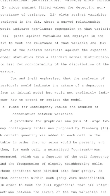
(e) Plots for Contingency Tables and Studies of Association between Variables

zero, each group of normalised contrasts was plotted separately on half-normal probability paper, assuming that the contrasts within each group formed an inde­ pendent sample from a normal distribution with zero mean and unit variance. Contrasts deviating signi­

ficantly from the theoretical unit variance line thus exhibited strong interaction. To separate the strong interaction contrasts from the rest, Fienberg used boundary lines suggested by Daniel {11} and Birnbaum {4} (see Figure 12). He pointed out that his pro­ cedure could be extended to handle the analysis of three-way tables and was a development of the pro­ cedure presented by Cox and Lauh (8), who adapted half-normal plotting to the analysis of contingency tables in which there was a binary response variable. A drawback to Cox and Lauh’s procedure was the fact that their plotted points were not independent, and thus the results for half-normal plotting were not strictly applicable.

CHAPTER 6

GRAPHICAL METHODS FOR GROWTH CURVES

Inspection of the preceding chapters reveals problem areas in which no work or very little work has been published concerning the application of graphical methods. One such problem area is growth curves. This is rather surprising since various methods of residual analyses have been successfully applied to model identification in regression studies and these studies have direct analogies in time

series models, which take the form of regression models with time as an independent variable.

One graphical approach for identification of growth curves has been advocated by Gregg, Hossell and Richardson {19}. The seven basic growth curves with their characterizing equations

are:-(i) Linear, y = a + bt,

(ii) Quadratic, y = a + bt * ct2 , (iii) Exponential, y = ae^^,

(iv) Logarithmic Parabola, y = a e ^ + ct 9

b t

(v) Simple Modified Exponential, y = K + ae ,

* ct_{D ©} (vi) Gompertz, y = ae

bt ~1 (vii) Logistic, y = (K + ae ) ,

where y denotes the growth variable, t denotes time,

and a, b, c and K are parameters.

The following relationships may easily be

(i) Linear, dy is constant, cTt

(ii) Quadratic, d£ = b + 2ct,

(iii) Exponential, d^ is constant,

(iv) Logarithmic Parabola, /l\ = b + 2ct

[yj

_at

(v) Simple Modified Exponential, log ^dy^ « log (ab) + bt,

(vi) Gompertz, log /I . d%\ = log (be) + ct, >y dtJ

and(vii) Logistic, log/1 . dy\ = log (-ab) + bt.

(7 *v

Using the word "slope” to mean the rate of change dy,

and estimating the value of y at any point by a moving average (m.a.), Gregg, Hossell and Richardson produced the table

below:-Compute and Plot Against

Time:-If the Plotted points vary about a straight line which

is:-Then the curve suggested

is:-Slope Horizontal Linear

Slope At an angle to the

horizontal Quadratic

Slope/m.a. Horizontal Exponential

SIope/m.a. At an angle to the horizontal

Logarithmic Parabola log(slope) Sloping down to

the right

Simple modified Exponential log(slope/m.a.) Sloping down to

the right

Gompertz

log jslope/ (m.a. f^J Sloping down to the right

The cjuantities in column 1 of the table, they lab­ elled ’’slope characteristics” and their procedure for identification was to plot the slope charac­ teristics of the data and inspect these plots for any indication of a satisfactory model.

This method has two practical difficulties

whose importance depends very much on the smoothness of the data available. There is first the problem of measuring the slopes at different times. This can be done approximately by taking first differen­ ces and smoothing these with a weighted moving aver­ age. Alternatively one can smooth first and then take differences or find the slope of a fitted trend line. Neither approach is very satisfactory. One can similarly question the use of a moving average to estimate the value of y at any point. The second problem comes from the fact that the method depends on an eye comparison of different plots to see which looks most like a straight line. One can, however, be misled in this since the vertical scales are all in different units.

are:-(a) Ay^ is constant for linear data, linear for quadratic data.

(b) Ay^ constant for exponential data. yt

t-1

^ is constant for linear, exponential Ayt-1 _{and simple modified exponential data.}

^ yt is constant for exponential and Ai°g yt_i

Gompertz data.

is constant for exponential

y

J and logistic data.

(f) Alog y^ is constant for exponential data,

linear for logarithmic parabola data. (s) *s constant for exponential data.

yt-l

Both these methods again depend on an eye comparison of different plots whose vertical scales are not

PART II

A GRAPHICAL IDENTIFICATION PROCEDURE

CHAPTER 7

FOUNDATION OF THE IDENTIFICATION PROCEDURE

Let the growth data we wish to identify be deno­ ted by Yi, Y2 Yn , the data being measured at equal intervals of time such that the value Y^ occurs at time t = i (i = 1,2,....n). The data is divided into overlapping "blocks11, each block consisting of a fixed number of consecutive data points, usually between 10 and 25 depending on the magnitude of n. The division is such that each block is comprised of an odd number of data points, say (2m+l), i.e. the k*th block, say, consists of data points Y^, Y^^,

....Yj,+ 2m with corresponding time base t = k, t = k+1,

.... t = k+2m (k = 1,2,....,n-2m). For convenience the time base of each B. is transformed into (2m+l) equally spaced points in the interval -l^x^+l. This is effected for by the transformation

which also has the property that the natural order of the original time base is preserved and further

kt**- -1 and k+2m «-*•+!. We shall use the notation 3j,

to denote the block B^ transformed by T^. To each block 3-,, we fit the model

where the ct^) are unknown parameters and gr (x) is a known polynomial of degree r in x which is fixed for the particular data under consideration. In deciding the value of h, the order of the polynomial fit, it was observed that too high a value results not only in computational difficulties but also in a relatively useless oscillatory fit to ’’noisy1’ data, itfhile smaller values yield a smoother fit and easier numerical handling. For example, Figure 13 illus­ trates quite well the difference in smoothness bet­ ween a seventh order and a fourth order polynomial fitted to a block of ’’noisy" exponential data. Tests such as that illustrated in Figure 13 together with computational algebraic difficulties encountered in the least squares process (see Chapter 8) led us to accept the value 4 for h as providing an acceptable level of smoothness of fit with a tolerable measure of algebraical and numerical manioulability.

(k)~(k) (k) (k) (k) Least squares estimates, aft, ai , a2, as, at*, (k) (k) (k) (k) (k)

of a0, ai , a2 , « 3 , respectively, are obtained

4-rM-J i 4-rM-J U ! 1 1 ' i '

rrr

f

L-U_4ft) LiJ J

taTl

+ t3C

"H

' ‘i ’"T'S i i jj j?

quadratic, exponential, logarithmic parabola, simple modified exponential, Gompertz and logistic.

Much choice is available for the polynomials gr (x) e.gj the Taylor series (so that gr (x) = xr), Legendre polynomials, Tchebychef polynomials etc. Each have their own particular advantages (and dis­ advantages) in fitting procedures. However, in our investigation the gr (x) are chosen in such a way as to attempt to minimise the ratios of the standard

00

deviations of the coefficients a. _{(j = 0,1,....4)}

to their absolute values, thus obtaining more reliable coefficient plots for identification purposes. While the full details are left until Chapter 10 it should be mentioned that such gr (x) are tailor-made to a particular set of data but are in no way block depen­ dent.

CHAPTER 8

THE LEAST SQUARES FITTING PROCESS

In this chapter the general form of the coe-(kj

fficients a^ (j = 0,1,...4) is obtained by the method of least squares. Throughout Part II of this thesis the notation | will denote summation over integer values from i = k to i = k+2m.

In the k fth block 8k, the data values are Yk, ^k+19 _{* * * *^k+2m corresP°nding x values xk = - m ,}

m xk+l " -

a i l

xk+2m = 2 » 50 that_m

Tk : t = k + i «-- ► x = xk+i = - m-i m To the block $k we fit the model

r=4 (k)

f (xi) = ZL «r gr Cxi) , (i » k,k+l,...k+2m), r=o

where

jjr (r) .

~ % _{pr-i xi} 9 ^ _~

j =o J

the p's being constants whose values are eventually 00

found in our attempt to minimise S.Dev, (a^ ) (k) ai

(j = 0,1,....4) for the data under consideration. We make the assumptions that Var(Y|x=x^) = crz,

The least squares estimates a^ ) 9 _{af^ ... .af^) of}

apc^, # o are those values of aPc^ , af^ .... which minimise the quantity

<Yi

r*=4

21 ciyk^ gjCxj))2. r=o

If g(r,s) = I _{gr(xf) * gsCxi), then least squares}

theory gives

g (0,0) g (0,1) g (0,4) gd,0)

g(4,0) g ( 4 , 4 )

a a a a a flO a (k) (k) (k) 2Yi gjfxj) f i

f i M xi)

P i

The calculation of the g(r,s) terms is given in Appendix 1. The inversion process for this matrix

is simplified by

(1) (2) (3) (3) (4) (i) putting the terms Pi , , px , p3 p,

(

4

)

and (ii) omitting terms of smaller order than

_ 7

0(m ), so forming a "truncated" matrix from the original.

To check that these approximations did not sig nificantly affect the matrix elements a programme X'ras written to calculate the elements of the ori­ ginal matrix above and the "truncated" matrix for values of m from 5 to 13. For convenience the p ’s were arbitrarily given Taylor series values i.e.

C j)

Ci)

pQ = 1, pr = 0 (r f 0) ; j =0,1,--- 4. A typical result (m = 7)

was:-QRIGINAL {g(r,s)} MATRIX

15.0 5.71428 3.89504 0 5.71428 0 3.89504 0 5.71428 0 3.89504 0 3.14178 0 3.89504 0 3.14178 0 3.89504 3.14178 2.74317

TRUNCATED FORM OF {g(r,s)} MATRIX

15.0 5.71428 3.89524 0 5.71428 0 3.89524 0 5.71428 0 3.89524 0 3.14275 0 3.89524 0 3.14275 0 3.89524 3.14275 2.74587

to truncation was 0.01%, a clearly acceptable figure. Similarly

The inverse of the truncated (g(r,s)} matrix is given in Appendix 2. To check the working, a pro­ gramme was written to compare this inverse with the inverse of the original {g(r,s)> matrix obtained by a Fortran subroutine, for values of m from 5 to 13 using Taylor series p values.

A typical result (m=7)

wast-INVERSE OF TRUNCATED (g(r,s)} MATRIX AS AS IN APPENDIX 2

0.237970 0 -1.01195 0 0.818274 0 1.12743 0 -1.39738 0 -1.01195 0 7.64035 0 -7.30850 0 -1.39738 0 2.05002 0 0.818274 0 -7.30850 0 7.57098

/

INVERSE OF ORIGINAL { g ( r , s ) } MATRIX USING

FORTRAN SUBROUTINE

0 -1.01132 0 0.818284

1.12946 0 -1.40025 0

0 7.64143 0 -7.31582

-1.40025 0 2.05426 0 0 -7.31582 0 7.58154

The largest error in an element is 0.14%. The errors increase with increasing values of m but at a declin­ ing rate. The largest error for m = 13 is 0.94%, an acceptable figure.

239449

-1.01132

0.81824

-Denoting the elements of the inverse of the truncated form of the {g(r,s)} matrix by G(r,s)

(r=0,l,... .4 ; si=o,l,... .4) , a good approximation

00

00

to the coefficients ao , ... a«» is given by

a o ^ \ / g( 0 , 0 ) G(0,1 ) ... G ( 0 , 4 ) \

00

aj (k) a2

(k) a3

(k) a*

G (1 , 0 )

G (4 ,0 ) ...G (4, 4)

(0)

?Yi P»

I

?Y. po x.

I C2)1 o (2) ?Y. (p0 x,2 + p2 )

(3) (3) ?Y. (po x.* + p2 x.)

r O ) \ ( O „ C4) /

jYj (Po + P2 Xj2+ Pk )/

(

.

)

where

00

Varfa^ ) = G(j,j) . o2, 0=0,1,...4)... (8.2)

-CHAPTER 9

PLOTS FOR MODEL IDENTIFICATION

In the following sections growth curve models are investigated in order to build up plotting pro­ cedures from the ’’sliding block” technique described in Chapter 7. The procedures are then inspected to see if one in particular would suffice for the identifi­ cation of the seven basic models.

(a) Linear Data

If the data under inspection was perfectly linear, then, at time t, Yt = a + bt where a and b are unknown parameters. Applying the transforma­ tion to the block we put t = mx + k + m, whence

in 6i<:

Y. = a+b(mx^+k+m) * (a+bk+bm)+bmx^,(i=k,k+l,...k+2m). To this data we are fitting the model

f (x.) = a0 po-°^+ai pJ1')xi+a2 (po^2^x|+p|2^) +

a3 (p^3-lx!+p|3^xi) + ak ^ _{(p£^x2+p|4-,x|+pit4')) ... (9.1)}

Equating coefficients we obtain, for non-zero PQ^ , Cj =09 _{1J • • *4)}

CIO CD

ax po = bm,

CD CO)

ao Po = a + bk + bm,

Ck) (k) CD

a 2 = as = = 0.

Ck)

In practice we replace the a. by their least squares

ck) * j

as aids to identifying linear

aata:-(i) A plot of ap^ against k would give a

straight line parallel to the k-axis having intercept bm

Po

(ii) A plot of aPc^ (vert.) against k (horiz.) would be linear, with slope b and

JO)

r V Pff

intercept /a+bm

(iii) A plot of a£^) agaiftst aP^ for increasing k would give a straight line perpendicular to the a£k) axis. The plotted points v/ould be equally spaced along this line.

(iv) A plot of a£k) against a|^ v/ould give a fkl

series of points along the a^ J _axis.

Similarly for against aP^ or a«P^. (v) A plot of apc^ against aPc^ (or ap^,aip))

fkl

would give a single point on the at _axis.

(b) Quadratic Data

If the data under inspection was perfectly quad­ ratic, then, at time t, = a + bt + ct2 where a,b

and c are unknown parameters. Transforming as in (a) we obtain for

= (a+bk+bm+ck2 +2ckm+cm2) + (bm+2ckm+2cm2) x^

+ cm2 x|, '(i = k,k+l,.. .lc+2m) .

Fitting model (9.1) and equating coefficients, we

-(j)

obtain, for non-zero po (i II o •#v • • /—\

(k)

ai _P0(2) = cm2 >

(k)

af P0(1) = bm + 2 c km + 2 cm2 ,

„cki

a o Po + a (k) + a2 p i J(2) = a + bk + bm

= a (k) k . 0

fk')

Replacement of the aj* by their least souares estimates J: .^suggests the following plots as aids to identifica­ tion:

-fkl

(i) A nlot of a2 against k would give a straight

line parallel to the k-axis having intercept cm2

p,(2 )

fkl

(ii) A plot of af“J _{(vert.) against k (horiz.)}

would be linear, with slope 2cm and

P0 (1>

intercept/bm+2cm2

Po (1>

(iii) A nlot of a<fk^ against a2k^ for increasing k would give a straight line perpendicular to the ai-^ axis.

(lO fkl

(iv) A plot of af J _{against a}2 would give a

straight line perpendicular to the a2k^ axis, the points being equally spaced along the line.

(v) A plot of af ^ against a3^ or a*k^ would give a series of equally spaced points along the a/k) axis.

(vi) A plot of against ap^ or a£k^ v/ould give a series of points along the aPc^ axis.

(c) Exponential Data

If the data under inspection was perfectly

expo-i * o .

nential, then, at time t, = a e where a and b are unknown parameters. Transforming as in (a) we obtain for B^:

Y. = a eM m x i+k+m) _

From (8.1) and Appendix 2,

a0(k) = G (0,0) ^YiPoCO) + G(0,2) E Y ^ P o ^ x U p P 5)

+ G(0,4) ZY, Cpo(4 )x p p2(4 :,x%p,(4))

X

Hence on substituting for Y^,

bmx.

a0(k) = G(0,0).pj0 b a . eb(k+m) Ze G(0,2) .a.eb(k+m)

i

?ebmXi (pf2>x?+pj2b ♦ GC0,4).a.eb <k«“ >

1 X X

(po^4 -*Xi+pl4^x?+p^4b »

i.e. a„(k) = a.eb fk+m) Ze bmx.1 (G(O,O)p0(O)+G(Of2)p2(2:) +

G(0,4)p^4b + Ze V (GCO,2)p0(2 )+G(O,4)p2(4b +

• X

r . bmx.

*e xiG(0,4)po(4)

Replacing x. by its value i-k-m and changing the var-m

form 2m

aebk Z _ebr{(G(0 ,0 )po(0)+G(0 ,2)p2(2)+G(0 ,4)p%(,!b +

r=o

fr - m2 (G(0.2)po(2:)->-G(0,4)p2(4)) + ,r-rK"G(0,4)p0(4)> ,

m } _{k m} J

ai-k+1^ b

whence it is easily seen that 0 * e , a

con-- 3 F “ stant.

a (k+1> b

Similarly it can be shown that _j = e (j*1,2,3,4). aj }

From (8.1) and Appendix 2 we may similarly derive the relationships:

ai(k) = aebk Z™

(G(l,l)p0(1)+ G ( l , 3 ) p P )) + frzm 1 s

r=o 1 m }

G(l,3)p0(3)} ,

a|k^ = a ebk z” ebr{ (G(2,0)p0(O)+G(2,2)p2(2)+G(2 ,4)pPb

r=o

+ .r-m 2 (G(2.2)p,(2)*GC2.4)p2C4h * fr-m »G(2.4)p,(4)} .

m ^ m '

(k) bk 2m

ajw s a e Z ebr{ (G(3,l)p0(1)tG(3,3)pPh*fr-m.

r=o k m '

G(3,3)po(3h .

ap) = a ebk z" 1 ebr{ (G (A ,O)p0(O)+G (4 ,2)p|2)+G (4 ,4)pJ4 5 )

r=o

fT ^1 2 (G(4,2)p0(2 )+G(4J4)p2(4)) + frIm1 ,tG(4,4)p0(4)}

^ m J 1 m '

.

(k)

It follows that c'r (r = 0,1,2,3,4; s = 0 ,1 ,2 ,3 ,4;

— m

as

r £ s) are constants whose values depend on m, b and the p terms.

The following plots would therefore be useful for identifying exponential

data:-(k+1 )

(i) Plots of aj against k (j = 0,1,2,3,4) j

would give a straight line parallel to the b

k-axis having intercept e .

(ii) Plots of against a^^ (r f s) would give straight lines passing through the origin. As k increases the plotted points become increasingly far apart along the lines.

(d) Simple Modified Exponential Data

If the data under inspection was perfectly simple modified exponential, then, at time t, = K + a e where a, b and K are unknown parameters. Transforming as in (a) we obtain for 3 ^:

From (8.1) and Appendix 2, it follows that

m COI b(mx.+k+m) ,,,

a0l J = G(0,0) Zp} J(K+ae 1 )+G(0,2) E(p0U J x|+

<-->1 b (mx. +l'+m) ,...

P2 ) (K+a6 1 ) + GCO,4) E(pol Jx H p_{i l l}2U J x? +

m b(mx.+k+m) pi ’')(K+ae

i.e. a£k) = k|g(OsO)po(0) (2m+l)+G(0,2) (pP^ Ex?+p|2)

i

(2m+l))+G(0,4) (Po4) Z x U p 2(4J

ZxUpi^

i i -*

+ a.eb(k+m) Ze bmx.1 (G(0,0)pf0)+G(0>2)p-i2)+G(0,4)pf4b

bmx. m bmx.

+ Ze x|(G(0,2)po ^+G(0 ,4)p2- -^) + Ze 1

G(0,4)pi£4) (9.2)

In Appendix 3 it is shown that the coefficient of K is non-zero.

Similar relationships may also be obtained for apv^, a|k^ , ap'*^ and ai^ f _{but these differ from a£k^}

in the essential feature that the coefficient of K is zero, a fact which is established in Appendix 3.

These results indicate that the following plots would be useful for identification of simple modi­

fied exponential data:-(k+1)

(i) Plots of aj against k (j = 1 ,2 ,3,4)