Munich Personal RePEc Archive
Unit Root Tests with Wavelets
Gencay, Ramazan and Fan, Yanqin
February 2007
Online at
https://mpra.ub.uni-muenchen.de/15913/
Unit Root Tests with Wavelets
∗
Yanqin Fan
†Ramazan Gen¸cay
‡First version: February 2007, This version: April 2009
Forthcoming in Econometric Theory
Abstract
This paper develops a wavelet (spectral) approach to testing the presence of a unit root in a stochastic process. The wavelet approach is appealing, since it is based directly on the different behavior of the spectra of a unit root process and that of a short memory stationary process. By decomposing the variance (energy) of the underlying process into the variance of its low frequency components and that of its high frequency components via the discrete wavelet transformation (DWT), we design unit root tests against near unit root alternatives. Since DWT is an energy preserving transformation and able to disbalance energy across high and low frequency components of a series, it is possible to isolate the most persistent component of a series in a small number of scaling coefficients. We demonstrate the size and power properties of our tests through Monte Carlo simulations.
Keywords: Unit root tests, discrete wavelet transformation, maximum overlap wavelet transformation, energy decomposition.
JEL No: C1, C2, C12, C22, F31, G0, G1.
∗This is a substantially shortened version of the paper: “Unit root and cointegration tests with wavelets.”
We are grateful to Pentti Saikkonen and two anonymous referees for detailed comments on the early paper which have helped improve the presentation of the results in the current paper. We also thank Stelios Bekiros, Buz Brock, Russell Davidson, Cees Diks, Cars Hommes, Benoit Perron, Hashem Pesaran, James MacKinnon, James Ramsey, Alessio Sancetta, Mototsugu Shintani and Zhijie Xiao for helpful discussions. All errors belong to the authors.
†Department of Economics, Vanderbilt University, VU Station B #351819, 2301 Vanderbilt Place,
Nashville, TN 37235-1819, U.S.A. Part of the work in this paper was done when Fan visited the Department of Economics at Simon Fraser University whose hospitality and support are acknowledged. Yanqin Fan is grateful to the National Science Foundation for research support. Email: [email protected]
‡Department of Economics, Simon Fraser University, 8888 University Drive, Burnaby, British Columbia,
1
Introduction
As Granger (1966) pointed out, the vast majority of economic variables, after removal of any trend in mean and seasonal components, have similar shaped power spectra where the power of the spectrum peaks at the lowest frequency with exponential decline towards higher frequencies. Since Nelson and Plosser (1982) argued that this persistence was captured by modeling the series as having a unit autoregressive root, designing tests for unit root has attracted the attention of many researchers. The well-known Dickey and Fuller (1979) unit root tests have limited power to separate a unit root process from near unit root alternatives in small samples. Phillips (1986) and Phillips (1987a) pioneered the use of the functional central limit theorem to establish the asymptotic distribution of statistics constructed from unit root processes. To construct unit root tests with serially correlated errors, one approach is due to Phillips (1987a) and Phillips and Perron (1988) by adjusting the test statistic to take account for the serial correlation and heteroskedasticity in the disturbances. The other approach is due to Dickey and Fuller (1979) by adding lagged dependent variables as explanatory variables in the regression. Other important contributions are Chan and Wei (1987), Park and Phillips (1988), Park and Phillips (1989), Sims et al. (1990), Phillips and Solo (1992) and Park and Fuller (1995). In general, unit root tests cannot distinguish highly persistent stationary processes from nonstationary processes and the power of unit root tests diminish as deterministic terms are added to the test regressions. For maximum power against very persistent alternatives, Elliottet al.(1996) (ERS) use a framework similar to Dufour and King (1991) (DK) to derive the asymptotic power envelope for point-optimal tests of a unit root under various trend specifications. Ng and Perron (2001) exploits the finding of ERS and DK to develop modified tests with enhanced power subject to proper selection of a truncation lag.
Most existing unit root tests make direct use of time domain estimators of the coefficient of the lagged value of the variable in a regression with its current value as the dependent variable, except Choi and Phillips (1993), the Von Neumann variance ratio (VN) tests of Sargan and Bhargava (1983) and their extensions. Recently, Cai and Shintani (2006) provide alternative VN tests based on combinations of consistent and inconsistent long run variance estimators. Phillips and Xiao (1998) and Stock (1999) provide a helpful review of the main tests and an extensive list of references.
relative to the overall variance of the process. If a particular band contributes substantially more to the overall variance relative to another frequency band, it is considered an important driver of this process. Recall that the spectrum of a unit root process is infinite at the origin, and hence the variance of a unit root process is largely contributed by low frequencies. By decomposing the variance1 of the underlying process into the variance of its low frequency
components and that of its high frequency components via the discrete wavelet transforma-tion (DWT), we design wavelet-based unit root tests. Since DWT is an energy preserving transformation and able to disbalance energy across high and low frequency components of a series, it is possible to isolate the most persistent component of a series in a small number of coefficients referred to as the scaling coefficients. Our tests utilize the scaling coefficients of the unit scale. In particular, we construct test statistics from the ratio of the energy from the unit scale to the total energy (variance) of the time series. We establish asymptotic properties of our tests, including their asymptotic null distributions, consistency, and local power properties. Our tests are easy to implement, as their asymptotic null distributions are nuisance parameter free and the corresponding critical values can be tabulated. The Monte Carlo simulations are conducted to compare the empirical size and power of our tests to the Dickey and Fuller (1979) (ADF), Phillips and Perron (1988) (PP), Elliottet al. (1996) (ERS) and Ng and Perron (2001) (MPP) tests. Our tests have good size and comparable power against near unit root alternatives in finite samples.
Choi and Phillips (1993) developed unit root tests based on an alternative spectral ap-proach to time series analysis, the Fourier spectral analysis, and demonstrated advantages of their tests over tests based on time domain approach. Unlike our tests, however, their tests make use of frequency domain estimators of the autoregressive coefficient. The DWT is an orthonormal transformation which may be relaxed through an oversampling approach termed as the maximum overlap DWT (MODWT), see, for example, Percival and Mofjeld (1997).2 The VN tests of Sargan and Bhargava (1983) are based on the ratio of the sample
variance of the first differences and the levels of the time series. These tests avoid the problem of redundant trend to gain efficiency. Sargan and Bhargava (1983) suggested using the VN statistic for testing the Gaussian random walk hypothesis, and Bhargava (1986) extended to the case of the time trend. Stock (1995) studied unit root tests with a linear time trend and Schmidt and Phillips (1992), working with polynomial trends, showed that the Lagrange multiplier principle leads to a VN test. Interestingly, we show that the VN tests are special
1
In the signal processing literature, the variance of a process is referred to as the energy of the process. In this paper, we use the two terminologies interchangeably.
2
cases of our wavelet tests when we use the Haar wavelet filter and unit scale MODWT. The Haar wavelet filter is the member of Daubechies compactly supported wavelet filter of the shortest length. By using Daubechies wavelet filter of longer length, our tests gain power over the VN tests in finite samples.
(2004).
This paper provides another context in which the use of the wavelet (spectral) approach may have advantages over the time domain approach or the Fourier approach. Unlike Hong (2000), Hong and Lee (2001), Lee and Hong (2001), Duchesne (2006a), Duchesne (2006b), and Hong and Kao (2004) who develop and/or make use of wavelet estimators of spectral density functions of the relevant processes, we employ directly the DWT of the observed time series. We contribute to the unit root literature on three different fronts. First, we propose a unified wavelet spectral approach to unit root testing; second, we provide a spectral interpretation of existing VN unit root tests; and finally, we propose higher order wavelet filters to capture low-frequency stochastic trends parsimoniously and gain power against near unit root alternatives.
In section two, we begin with a brief overview of wavelets, discrete wavelet filters and discrete wavelet transformation. In section three, we develop our wavelet-based unit root tests against purely stationary alternatives and trend stationary alternatives. Section four provides Monte Carlo simulations on the size and power properties of our tests. We conclude thereafter. An appendix contains technical proofs. Throughout this paper, we use =⇒ to denote weak convergence. All the limits are taken as the sample size approaches ∞.
2
Discrete Wavelet Transformation
A wavelet is a small wave which grows and decays in a limited time period.3 To formalize
the notion of a wavelet, let ψ(.) be a real valued function such that its integral is zero, R∞
−∞ψ(t)dt = 0, and its square integrates to unity,
R∞ −∞ψ(t)
2dt = 1. Thus, although ψ(.)
has to make some excursions away from zero, any excursions it makes above zero must cancel out excursions below zero, i.e.,ψ(.) is a small wave, or a wavelet.
Fundamental properties of the continuous wavelet functions (filters), such as integration to zero and unit energy, have discrete counterparts. Leth = (h0, . . . , hL−1) be a finite length
discrete wavelet (or high pass) filter such that it integrates (sums) to zero, PL−1
l=0 hl = 0,
and has unit energy, PL−1
l=0 h2l = 1. In addition, the wavelet filterh is orthogonal to its even
shifts; that is,
L−1
X
l=0
hlhl+2n = ∞
X
l=−∞
hlhl+2n= 0, for all nonzero integersn. (1)
The natural object to complement a high-pass filter is a low-pass (scaling) filterg. We will denote a low-pass filter asg = (g0, . . . , gL−1). The low-pass filter coefficients are determined
3
This section closely follows Gen¸cayet al.(2001), see also Percival and Walden (2000). The contrasting
by the quadrature mirror relationship4
gl = (−1)l+1hL−1−l for l= 0, . . . , L−1 (2)
and the inverse relationship is given byhl = (−1)lgL−1−l. The basic properties of the scaling
filter are: PL−1 l=0 gl =
√
2, PL−1
l=0 g2l = 1, L−1
X
l=0
glgl+2n= ∞
X
l=−∞
glgl+2n= 0, (3)
for all nonzero integersn, and
L−1
X
l=0
glhl+2n = ∞
X
l=−∞
glhl+2n= 0 (4)
for all integers n. Thus, scaling filters are average filters and their coefficients satisfy the orthonormality property that they possess unit energy and are orthogonal to even shifts.
By applying both h and g to an observed time series, we can separate high-frequency oscillations from low-frequency ones. Let y = {yt}Tt=1 be a dyadic length vector (T = 2M)
of observations where M = log2(T). The length T vector of discrete wavelet coefficients w
is obtained by w = Wy, where W is a T ×T real-valued orthonormal matrix defining the DWT which satisfies WTW = I
T (T ×T identity matrix). We refer the interested reader
to Percival and Walden (2000) for a detailed discussion on the construction of W from the wavelet and scaling filters. The vector of wavelet coefficients may be organized into M + 1 vectors,
w = [w1,w2, . . . ,wM,vM]T, (5)
where wj is a length T /2j vector of wavelet coefficients associated with changes on a scale
of length λj = 2j−1 and vM is a length T /2M vector of scaling coefficients associated with
averages on a scale of length 2M = 2λ M.
In practice the DWT is implemented via a pyramid algorithm of Mallat (1989, 1998). The first iteration of the pyramid algorithm begins by filtering (convolving) the data with each filter to obtain the unit-scale wavelet and scaling coefficients:
Wt,1 =
L−1
X
l=0
hly2t−lmodT and Vt,1 = L−1
X
l=0
gly2t−lmodT,
4
where t = 1, . . . , T /2. Let w1 = W1,1, ..., WT /2,1
′
and v1 = V1,1, ..., VT /2,1
′
denote respec-tively the vectors of unit-scale wavelet and scaling coefficients. We obtain the level 1 partial DWTw = [w1, v1]T.
The second step of the pyramid algorithm starts by defining the “data” to be the scaling coefficientsv1 from the first iteration and apply the filtering operations as above to obtain
the second level of wavelet and scaling coefficients:
Wt,2 =
L−1
X
l=0
hlV2t−l,1 modT /2 and Vt,2 = L−1
X
l=0
glV2t−l,1 modT /2,
t = 1, . . . , T /4. Keeping all vectors of wavelet coefficients, and the final level of scaling co-efficients, we have the following length T decomposition w = [w1, w2, v2]T, where w2, v2
denote respectively the vectors of second scale wavelet and scaling coefficients. This proce-dure may be repeated up to M times where M = log2(T) and gives the vector of wavelet coefficients in Equation (5).
The orthonormality of the matrix W implies that the DWT is a variance preserving transformation:
kwk2 =
T /2M X
t=1
Vt,M2 +
M
X
j=1
T /2j X
t=1
Wt,j2 =
T
X
t=1
y2t =kyk2 .
This can be easily proven through basic matrix manipulation via
kyk2 =yTy= (Ww)TWw =wTWTWw =wTw =kwk2
.
Given the structure of the wavelet coefficients,kyk2 is decomposed on a scale-by-scale basis via
kyk2 =
M
X
j=1
kwjk2+kvMk2, (6)
where kwjk2 = PT /2
j
t=1 Wt,j2 is the sum of squared variation of y due to changes at scale λj
and kvMk2 =PT /2
M
t=1 Vt,M2 is the information due to changes at scales λM and higher.
The idea behind our wavelet unit root tests can be best understood through the energy (variance) decomposition of a white noise process and that of a unit root process. To illustrate, in Figure 1, the dot chart of a Gaussian white noise process is plotted for 1024 observations (M = 210 = 1024). A six level (J = 6)5 DWT is used. “Data” represents the
total energy of the data which is normalized at one, wi, i= 1, . . . ,6 represents the percentage energy of wavelet coefficients, and v6 is the percentage energy of the scaling coefficients. The
5
sum of the energies of the wavelet and the scaling coefficients is equal to the total energy of the data. The energy is the highest at the highest frequency wavelet coefficient (w1) and declines gradually towards the lowest frequency wavelet coefficient (w6). The percentage energy of the scaling coefficient (v6), i.e.,kvJk2/kyk2, is close to zero. In Figure 2, the dot
chart of a unit root process
yt=yt−1+ut, ut ∼i.i.d. N(0,1) (7)
is plotted for y0 = 0 and t = 1,2, . . . ,1024 observations. The energy is the highest for the
scaling coefficients and almost zero at all wavelet coefficients. The percentage energy of the scaling coefficients (v6), i.e.,kvJk2/kyk2, is almost equal to one. The number of coefficients
needed equals 41 (41/1024 = 4%) of the total number of coefficients to account for almost all energy of the data. Heuristically, when a white noise process is added up (say, as in a unit root process), the high frequencies are smoothed out (those spikes in the white noise disappear) and what is left is the long term stochastic trend. On the contrary, when we do differencing (e.g., first differencing to a unit root, then we are back to the white noise series), we get rid of the long term trend, and what is left is the high frequencies (spikes) with mean zero. Since a unit root process can be succinctly approximated by a few scaling coefficients and the energy of the scaling coefficients is almost equal to the total energy of the data, we develop our statistical tests for a unit root process based on this principle of energy decomposition.
3
New Unit Root Tests
Let{yt}Tt=1 be a univariate time series generated by
yt =ρyt−1+ut, (8)
where {ut} is a weakly stationary zero-mean error with a strictly positive long run variance
defined by ω2 ≡ γ
0 + 2P
∞
j=1γj where γj = E(utut−j). Throughout this paper, the initial
condition is set toy0 =Op(1) and the following assumption on the error term is maintained.
Assumption 1:
(a) {ut}is a linear process defined asut=ψ(L)ǫt=P ∞
j=0ψjǫt−j, ψ(1)6= 0,and
P∞
j=0j|ψj|<
∞;
(b) {ǫt} is i.i.d. with E(ǫt) = 0, V ar(ǫt) =σ2, and finite fourth cumulants, and ǫs = 0 for
The last condition in Assumption 1(a) is referred to as 1-summability of ψ(L). The as-sumptionǫs = 0 fors ≤0 in Assumption 1(b) is made for convenience. Under Assumption 1,
we haveω2 =ψ(1)2σ2 andT−1/2P[T·]
t=1ut =⇒ ωW(·) where [T r] denotes the integer part of
T randW(·) denotes a standard Brownian motion defined onC[0,1], the space of continuous functions on [0,1]. It is known that the weak convergence result: T−1/2P[T·]
t=1ut =⇒ ωW(·)
holds for more general/other classes of processes than the class of linear processes specified in Assumption 1 including linear processes with martingale difference innovations {ǫt}, see
Phillips and Solo (1992). One may also extend the weak convergence result to linear pro-cesses with GARCH innovations by making use of the weak convergence result for GARCH processes, see Berkes et al. (2008). It is possible to extend the results to be developed in this paper to these other processes. For ease of exposition, we will stick to Assumption 1 in this paper.
In Subsections 3.1 and 3.2, we consider tests for H0 : ρ = 1 against H1 : |ρ| <1 in (8).
Under the alternative hypothesis, {yt} is a zero-mean stationary process with the long run
variance ω2/(1 −ρ)2. As mentioned in Section 2, our tests for unit root are based on the
different behavior of the energy decomposition of a unit root process and that of a short-memory such as a white noise process. To introduce the fundamental idea, we first develop a test based on the Haar wavelet filter and unit scale DWT in Subsection 3.1. In Subsection 3.2, we extend it to tests based on any Daubechies (1992) compactly supported wavelet filter of finite length. Finally, we extend the tests developed in Subsections 3.1 and 3.2 to trend stationary alternatives in Subsection 3.3.
3.1
The first test — Haar wavelet filter
Consider the unit scale Haar DWT of {yt}Tt=1 where T is assumed to be even. The wavelet
and scaling coefficients are given by
Wt,1 =
1
√
2(y2t−y2t−1), t= 1,2, . . . , T /2, (9) Vt,1 =
1
√
2(y2t+y2t−1), t= 1,2, . . . , T /2. (10) The wavelet coefficients {Wt,1} capture the behavior of {yt} in the high frequency band
[1/2,1], while the scaling coefficients{Vt,1}capture the behavior of{yt}in the low frequency
band [0,1/2]. The total energy of {yt}Tt=1 is given by the sum of the energies of {Wt,1} and
{Vt,1}. Since for a unit root process, the energy of the scaling coefficients{Vt,1} dominates
that of the wavelet coefficients {Wt,1}, we propose the following test statistic:
ˆ ST,1=
PT /2
t=1Vt,21
PT /2
t=1Vt,21+
PT /2
t=1Wt,21
Heuristically, underH0, ˆST,1 should be close to 1, sincePtT /=12Vt,21 dominates
PT /2
t=1Wt,21, while
under H1, ˆST,1 should be smaller than 1. We formalize these statements in the following
lemma.
Lemma 3.1 Under H0, SˆT,1 = 1 +op(1), while under H1, SˆT,1 = E(y2t+y2t−1)
2
E(y2t+y2t−1)
2
+E(y2t−y2t−1)
2 +
op(1).
Note that:
E(y2t+y2t−1)2
E(y2t+y2t−1)2+E(y2t−y2t−1)2
= E V
2
t,1
E V2
t,1
+E W2
t,1
<1.
We conclude that it is the relative magnitude of the energy of the scaling coefficients to that of the wavelet coefficients that determines the power of the test based on ˆST,1 and we expect
our test based on ˆST,1 to have power against H1.
The asymptotic distribution of ˆST,1 under H0 is summarized in the following theorem.
Theorem 3.2 Under H0, T( ˆST,1−1) =⇒ −λ2 γ0
v
R1 0[W(r)]
2dr, where λ
2
v = 4ω2.
The proof of Theorem 3.2 in the Appendix makes it clear that it is the energy of the scaling co-efficients that drives the asymptotic behavior of ˆST,1 under the null hypothesis. Alternatively,
noting the energy decomposition:PT /t=12V2
t,1+
PT /2
t=1Wt,21 =
PT
t=1yt2, we get immediately,
T( ˆST,1−1) = −
T−1PT /2
t=1 Wt,21−EWt,21
T−2PT t=1yt2
−
1 2EW
2
t,1
T−2PT t=1yt2
= − op(1) ω2R1
0[W(r)]2dr
− γ0
4ω2R1
0[W(r)]2dr
= − γ0 λ2
v
R1
0[W(r)]2dr
+op(1) under H0.
There are two unknown parameters in the asymptotic null distribution of ˆST,1: γ0 =
E(u2
2t) and λ2v or ω2. To estimate these parameters, we let ˆut = yt−ρyˆ t−1 denote the OLS
residual. Then ˆγ0 =T−1PtT=1uˆ2t is a consistent estimator of γ0. Being the long run variance
of {ut}, ω2 can be consistently estimated by a nonparametric kernel estimator with the
Bartlett kernel:
b ω2 = 4ˆγ
0 + 2
q
X
j=1
[1−j/(q+ 1)]ˆγj,
where q is the bandwidth/lag truncation parameter and ˆγj =T−1PTt=j+1uˆtuˆt−j, see Newey
and West (1987).6 Andrews (1991) showed that this long run variance estimator is consistent
6
Newey and West (1987) suggest setting the bandwidth using the sample size dependent rule of 4(T /100)2/9
when the bandwidth q grows at a rate slower than T1/2, with an optimal growth rate being
T1/3 under some moment conditions. Let ˆλ2
v = 4ωb2 and define the test statistic as
F G1 =
Tˆλ2
v
ˆ γ0
h ˆ ST,1−1
i .
Then under the null hypothesis, the limiting distribution of the test statistic F G1 is given
by the distribution of
−R1 1 0[W(r)]2dr
.
The limiting distribution of F G1underH0 is free from nuisance parameters and is extremely
easy to simulate, see MacKinnon (2000) for a detailed treatment. The critical values of this test are tabulated in the first row of Table 1.
We note that an alternative way to estimate γ0 is via the wavelet variance estimators.
We will elaborate on this approach in the next subsection when we allow the use of a general filter. Also, ω2 can be estimated by any existing long run variance estimators, including the
wavelet-based estimator of Hong (2000).
3.2
A general test — Daubechies compactly supported wavelet
filter
For a general Daubechies compactly supported wavelet filter{hl}L −1
l=0 , the boundary-independent
(BI) unit scale wavelet and scaling coefficients are given by
Wt,1 =
L−1
X
l=0
hly2t−l, Vt,1 = L−1
X
l=0
gly2t−l, (12)
where t=L1, L1+ 1, . . . , T /2 with L1 =L/2. Again the wavelet coefficients{Wt,1} extract
the high frequency information in {yt}. Since any Daubechies wavelet filter has a difference
filter embedded in it,{Wt,1} is stationary under both H0 and H1. However the sequence of
scaling coefficients{Vt,1}, extracting the low frequency information in {yt}, is nonstationary
under H0 and stationary under H1. Reflected in their respective energies, this implies that
the energy of the scaling coefficients dominates that of the wavelet coefficients under H0,
which forms the basis for our tests. Define7
ˆ ST,L1 =
PT /2
t=L1V
2
t,1
PT /2
t=L1V
2
t,1+
PT /2
t=L1W
2
t,1
.
We will construct a test for unit root based on the following asymptotic properties of ˆSL T,1.
7
Theorem 3.3 (i) SˆL
T,1 = 1 +op(1) under H0 and SˆT,L1 = cL +op(1) under H1 with cL = E(V2
t,1)
E(V2
t,1)+E(W 2
t,1)
<1; (ii) T2( ˆSL
T,1−1) =⇒ −
E(W2
t,1)
λ2
v
R1 0[W(r)]
2dr under H0.
Theorem 3.3(i) implies that a consistent test for unit root can be based on ˆSL
T,1.
Theo-rem 3.3(ii) extends TheoTheo-rem 3.2 from the Haar filter (L= 2) to any Daubechies compactly supported wavelet filter of finite length L. Since as the length of the filter L increases, the approximation of the Daubechies wavelet filter to the ideal high-pass filter improves8, we
expect tests based on ˆST,L1 to gain power as L increases. On the other hand, as L increases, the number of BI wavelet and scaling coefficients will decrease which would have an adverse effect on the power of our tests. It might be possible to choose L based on some power criterion function, but this is beyond the scope of this paper. In other applications of DWT with Daubechies compactly supported wavelet filter, L= 2 or 4 are often used.
Note that E W2
t,1
equals twice of the so-called wavelet variance at the unit scale. As a result, existing wavelet variance estimators can be used to estimate E W2
t,1
, see Percival (1995) for a detailed comparison of the wavelet variance estimators based on DWT and MODWT respectively. Based on DWT, 2υb2
y,1is a consistent estimator of the wavelet variance,
where
b
υy,21 = 1
(T /2−L1+ 1)
T /2
X
t=L1
Wt,21. (13)
Define the test statistic:
F GL1 = T 2
! ˆ λ2
v
b υ2
y,1
h ˆ
ST,L1−1i.
Under the null hypothesis, the limiting distribution of F GL
1 is the same as that ofF G1.
We now develop asymptotic power functions for our unit root tests by considering the sequence of local alternatives given by
ρ= expc T
∼1 + c
T (14)
for a particular value of c < 0. Under this sequence of local alternatives, it is well known that
T−2 T
X
t=1
yt2 =⇒ ω2 Z 1
0
[Jc(r)]2dr,
where
Jc(r) =
Z r
0
exp{(r−u)c}dW(u)
is the Ornstein-Uhlenbeck process generated in continuous time by the stochastic differential equationdJc(r) =cJc(r)dr+dW(r). Using this, one can easily show that under this sequence
8
of local alternatives, the asymptotic distributions of the test statistics F GL
1,F G1 are of the
same form as those under the null hypothesis except that the Brownian motion W(·) is replaced with the Ornstein-Uhlenbeck process Jc(·), i.e., −1/
R1
0 [Jc(r)] 2
dr. In particular, this leads to the conclusion that all these tests have the same asymptotic power (to the first order) against the sequence of local alternatives of the form (14). The following theorem states consistency and local power properties of our tests.
Theorem 3.4 (i) Under H1, Pr F GL1 <−C
→ 1 for any fixed positive constant C; (ii)
Under (14), we obtain:
F GL1 =⇒ −R1 1
0[Jc(r)]2dr
.
3.3
Tests against trend stationarity
Tests developed in the previous subsections can be extended to deal with trend stationary alternatives. We adopt the components representation of a time series and work with the detrended series, see Schmidt and Phillips (1992), Phillips and Xiao (1998), and Stock (1999). For ease of exposition, we restrict ourselves to non-zero mean and linear trend cases only. Phillips and Xiao (1998) also have a detailed discussion on efficient detrending for general trends.
The process {yt}is assumed to be of the form:
yt=µ+αt+yts, (15)
where {yst} is generated by model (8). Under H0 :ρ = 1, {yst} is a unit root process while
under H0 : |ρ| < 1, {yst} is a zero mean stationary process. If α = 0, we consider the
demeaned series {yt−y}, where y =T−1PTt=1yt is the sample mean of {yt}. Ifα 6= 0, we
work with the detrended series neyt−ye
o
, where eyt=Ptj=1 ∆yj −∆yand yeis the sample
mean of {yet}, in which ∆yt = yt−yt−1 and ∆y is the sample mean of {∆yt}. Alternative
expressions for the detrended series nyet−ye
o
can be found in Schmidt and Phillips (1992). Let WM
t,1 and
VM
t,1 denote respectively the unit scale DWT wavelet and scaling
co-efficients of the demeaned series{yt−y}. We will construct our tests based on
b SLM
T,1 =
PT /2
t=1(Vt,M1)2
PT
t=1(yt−y)2
.
Similarly, letWd
t,1 and
Vd
t,1 denote respectively the unit scale DWT wavelet and scaling
coefficients of the detrended series neyt−ey
o
. We will construct our tests based on
b
ST,Ld1 =−
PT /2
t=1(Vt,d1)2
PT
t=1(eyt−y)e2
UnderH0,it is known thatT−2PtT=1(yt−y)2 =⇒ ω2
R1
0 [Wµ(r)] 2
dr and T−2PT
t=1(yet−
e
y)2 =⇒ ω2R1
0 [Vµ(r)] 2
dr, whereWµ(r) =W(r)−
R1
0 W(u)du andVµ(r) =V(r)−
R1
0 V(u)du
in which V(r) =W(r)−rW(1).
Theorem 3.5 UnderH0,we have: (i)T
b SLM
T,1 −1
=⇒ − E(Wt,M1) 2
2ω2R1 0[Wµ(r)]
2
dr;(ii)T
b SLd
T,1−1
=⇒
− E(Wt,d1) 2
2ω2R1 0[Vµ(r)]
2
dr. Under (14), we have: (i)T
b SLM
T,1 −1
=⇒ − E(Wt,M1) 2
2ω2R1 0[JcM(r)]
2
dr;(ii)T
b SLd
T,1−1
=⇒
− E(Wt,d1) 2
2ω2R1 0[Jcd(r)]
2
dr, whereJ
M c (r) =
Rr
0 exp{(r−u)c}dWµ(u)andJcd(r) =
Rr
0 exp{(r−u)c}dVµ(u).
To estimate ω2, we take the OLS residuals from a regression of y
t on a linear trend
and yt−1 and then apply a nonparametric kernel estimator with the Bartlett kernel to the
residuals.
Remark 3.1. It is interesting to note that when the Haar wavelet filter is used,
b
ST,LM1 = 1− PT /2
t=1(y2t−y2t−1)2/2
PT
t=1(yt−y)2
.
This expression resembles that of the Sargan and Bhargava (1983) and Bhargava (1986) test. In fact, we can obtain the Sargan and Bhargava (1983) and Bhargava (1986) test from an extension of SbLM
T,1 by using MODWT instead of DWT. To see this, we recall that apart from
a factor of √2, the unit scale MODWT wavelet and scaling coefficients of {yt−y}are given
by
f Wt,1 =
L−1
X
l=0
hlyt−lmodT, Vet,1 = L−1
X
l=0
gl(yt−lmodT −y), (16)
where t = 1, . . . , T. It is easy to see that the DWT coefficients are obtained from the corresponding MODWT coefficients via downsampling by 2. At each scale, there are T MODWT wavelet coefficients and T MODWT scaling coefficients. Let
e ST,LM1 =
PT t=1Vet,21
PT
t=1Vet,21+
PT t=1fWt,21
.
With the Haar wavelet filter, apart from one coefficientVe2
1,1 in the numerator, SeT,LM1 reduces
to
e
ST,LM1 = 1− PT
t=2(yt−yt−1)2
PT
t=1(yt−y)2
,
so that1−SeLM T,1
with the Haar wavelet filter is the VN ratio used in Sargan and Bhargava (1983).
Remark 3.2. Generalizing the local power properties ofF GL
1 in Theorem 3.4 (ii) to trend
the asymptotic distributions of the test statistics developed in this subsection are of the same form as those under the null hypothesis except that the Brownian motion is replaced with the Ornstein-Uhlenbeck processJM
c (·) whenα = 0 and withJcd(·) when α6= 0. This implies
that their asymptotic power is the same as that of Sargan-Bhargava test. Hence, the local power analysis provided in Elliott et al. (1996) (ERS) applies to our tests.
4
Monte Carlo Simulations
In this section, we investigate the finite sample performance of the new unit root tests against trend stationary alternatives and compare them against the Elliott et al. (1996) (ERS) and Ng and Perron (2001) (MPP) tests. To save space, we restrict ourselves to non-zero mean and linear trend cases only.9
The asymptotic critical values of tests based on SbLM
T,1 and SbT,Ld1 are tabulated in Table 1.
These critical values are calculated from one million replications. The simulations are carried out for a sample size of 1,000 observations and 5,000 replications. Under the alternative, we discard the first 1,000 observations as transients. We have purposely chosenρvalues of 0.99 and 0.98 to seek the power of the tests for very near unit root alternatives.
In Tables 2 and 3, we examine the size and power properties of the wavelet tests for b
SLM
T,1 and SbT,Ld1 with serially correlated errors. The error process is a stationary AR(1) with a
parameter (γ) in the range of -0.8, -0.5, 0, 0.5, and 0.8. We set the bandwidth for the long-run variance to 20 and 50 with the Bartlett kernel for the SbLM
T,1 andSbT,Ld1 tests to ensure that
the empirical sizes are close to their nominal ones across these ranges of serially correlated errors.10 As illustrated in Table 2, the wavelet test with demeaned series has higher power
relative to ERS and MPP tests when γ < 0. At the 5% level, γ = −0.8, and ρ = 0.99, the SbLM
T,1 , ERS and MPP tests have powers of 99.7%, 40.1% and 40.2%, respectively. For
γ = −0.5, ρ = 0.99, and at the 5% level, the SbLM
T,1 , ERS and MPP tests have powers of
87.1%, 39.6% and 39.3%, respectively. Whenγ <0, the contribution of the error persistence concentrates in higher frequencies and it becomes easier for the wavelet test to separate such persistence from low frequency ones. For γ > 0, the simulation results between three tests are in the same order of magnitude for up to γ= 0.5. For γ = 0.8, the ERS and MPP tests perform better for certain critical levels. This is partly due to the fact that the wavelet test under-rejects for our choice of the bandwith for γ = 0.8.
A similar type of performance comparison is observed in Table 3 for SbLd
T,1. The wavelet
9
In the following tables, we report empirical size and power and do not adjust the empirical power for slight variations in empirical size.
10
test does much better for γ < 0. For γ = −0.8, ρ = 0.99, and at the 5% level, the SbLd T,1,
ERS and MPP tests have powers of 100%, 39.9% and 39.9%, respectively. On the other hand, ERS and MPP tests do better than the wavelet test for γ = 0.5 and 0.8. For γ = 0.8, ρ = 0.99, and at the 5% level, the SbT,Ld1, ERS and MPP tests have powers of 15.6%, 42.1%
and 41.2%, respectively.
5
Conclusions
Our unit root tests provide a novel approach in disbalancing the energy in the data by con-structing test statistics from its lower frequency dynamics. We contribute to the unit root literature on three different fronts. First, we propose a unified wavelet spectral approach to unit root testing; second, we provide a wavelet spectral interpretation of existing Von Neumann variance ratio tests, and finally, we propose higher order wavelet filters to capture low-frequency stochastic trends parsimoniously and gain power against near unit root alter-natives in finite samples. In our tests, the intuitive construction and simplicity are worth emphasizing. The simulation studies demonstrate the comparable power of our tests with reasonable empirical sizes.
Several extensions of our tests are possible. First, our tests make use of the unit scale DWT only (J = 1) and hence of the energy decomposition of {yt} into frequency bands
Appendix: Technical Proofs
Proof of Lemma 3.1. Suppose H0 holds. Thenyt=yt−1+ut. Equations (9) and (10)
imply:
Wt,1 =
1
√
2u2t and Vt,1 = 1
√
2(2y2t−1+u2t). (17) Using Equation (17), together with Equation (11), we obtain
ˆ ST,1 =
PT /2
t=1Vt,21
PT /2
t=1Vt,21+12
PT /2
t=1u22t
, (18)
where
T /2
X
t=1
Vt,21 = 1 2{4
T /2
X
t=1
y22t−1+ 4 T /2
X
t=1
u2ty2t−1 + T /2
X
t=1
u22t} ≡2AT + 2BT +
1
2CT, (19)
in which AT = PT /t=12x2t, BT = PT /t=12u2txt, and CT = PT /t=12u22t with xt ≡ y2t−1 for t =
1,2, . . . , T /2.
Below, we show that under H0,
AT =Op(T2), BT =Op(T), CT =Op(T). (20)
LetT1 = T2. By Proposition 17.2 in Hamilton (1994), we have
xt=x0+
t
X
j=1
vt=x0+ 2t−1
X
j=0
uj =x0+
(
u0+ψ(1) 2t−1
X
j=1
ǫj+η2t−1−η0
) .
Define the partial sum process associated with{vt}as XT1(r) =
1
T1
P[T1r]
t=1 vt,0≤r≤1.Then
it follows that
XT1(r)
L
= 1 T1
ψ(1)
2[T1r]−1
X
j=1
ǫj = 2ψ(1)
1 T
[T r]−1
X
j=1
ǫj.
By the functional Central Limit Theorem (CLT), we obtain √T XT1(·) =⇒2ψ(1)σW(·).
Ob-serving that PT1
t=1x2t = T2 1 2 1 R 0 T X2
T1(r) dr,we obtain by the Continuous Mapping Theorem
(CMT), 1 T2 1 T1 X t=1
x2t =⇒ 1 2λ 2 v 1 Z 0
W2(r)dr,
where λv = 2ψ(1)σ. As a result, we get
T−2
1 AT =⇒
1 2 λ 2 v Z 1 0
We now look atBT.Recall thatBT =PT
1
t=1u2ty2t−1. Simple algebra shows that E(BT) =
1 2
PT−1
s=1(T −s −1)γs = O(T) and V ar(T
−1
BT) = o(1), where γj = σ2P ∞
s=0ψsψs+j, for
j = 0,1,2, . . .. HenceBT =Op(T). The order ofCT follows from the Law of Large Numbers
(LLN).
Hence under H0, we get PtT=11 Vt,21 =Op(T2) and PTt=11 Wt,21 = Op(T), implying that the
energy of the scaling coefficients dominates that of the wavelet coefficients as mentioned above. Consequently,
ˆ ST,1=
T−2PT1
t=1Vt,21
T−2
(PT1
t=1Vt,21+
PT1
t=1Wt,21)
= 1 +op(1). (22)
Now consider what happens under H1. In this case, |ρ| <1 so that yt =ρyt−1+ut and
{yt} is a stationary short memory process. Thus, under H1, both {Vt,1} and {Wt,1} are
stationary, short memory processes. Moreover,
2 T1 T1 X t=1 W2
t,1 =
1 T1 T1 X t=1 y2 2t+
1 T1 T1 X t=1 y2 2t−1−
2 T1
T1
X
t=1
y2ty2t−1 =
2γ0
1 +ρ +op(1),
implying PT1
t=1Wt,21 =Op(T). Similarly, we obtain PtT=11 Vt,21 = Op(T), since T21
PT1
t=1Vt,21 = 2γ0
1−ρ +op(1). As a result, we obtain
ˆ ST,1 =
T−1
1
PT1
t=1Vt,21
T−1
1
PT1
t=1Vt,21+T
−1
1
PT1
t=1Wt,21
= E(V
2
t,1)
E(V2
t,1) +E(Wt,21)
+op(1)
= E(y2t+y2t−1)
2
E(y2t+y2t−1)2+E(y2t−y2t−1)2
+op(1). (23)
Proof of Theorem 3.2. Under H0, we note that
ˆ
ST,1−1 =−
CT/2−T4γ0
2AT + 2BT +CT −
T
4γ0
2AT + 2BT +CT
,
where AT, BT, CT are defined in (19). Note that CT = PtT=11 u22t and E(CT) = T1E(u22t) =
T1γ0, in which γ0 = σ2P
∞
s=0ψ2s. We obtain T −1
1 CT −γ0 = op(1). This, (21), and the fact
that BT = Op(T) imply:
T1( ˆST,1−1) = −
T−1
1 CT/2− T21γ0
2T−2
1 (AT+BT +CT/2) −
1 2γ0
2T−2
1 (AT +BT+CT/2)
= − op(1) λ2
v
R1
0[W(r)]2dr
−
1 2γ0
λ2
v
R1
0[W(r)]2dr
= − γ0 2λ2
v
R1
0[W(r)]2dr
where λ2
v = 4ω2.
Proof of Theorem 3.3. (i) UnderH0 : ρ = 1. We now show that T
−1
1
PT1
t=L1W
2
t,1 =
E W2
t,1
+op(1) and T −2
1
PT1
t=L1V
2
t,1 =Op(1). Hence, under H0, we obtain
ˆ ST,L1 =
1
1 +
PT1
t=L1W 2
t,1
PT1
t=L1V 2
t,1
= 1 1 + Op(T)
Op(T2)
= 1 +op(1).
To show T−1
1
PT1
t=L1W
2
t,1 =E Wt,21
+op(1), we note:
Wt,1 =y2t+1−L L−1
X
l=0
hl+ L−2
X
l=0
hl
(L−2−l
X
j=0
u2t−j−l
) =
L−2
X
l=0
hl
(L−2−l
X
j=0
u2t−j−l
) ,
implying thatWt,1is a finite linear combination of{ut}. The claim follows immediately from
Assumptions 1 and 2.
Now we consider the order of PT1
t=L1 V
2
t,1. Noting that
Vt,1 =y2t+1−L L−1
X
l=0
gl+ L−2
X
l=0
gl
(L−2−l
X
j=0
u2t−j−l
)
=√2y2t+1−L+ L−2
X
l=0
gl
(L−2−l
X
j=0
u2t−j−l
) , we obtain 1 T2 1 T1 X
t=L1
Vt,21 =
1 T2
1
T1
X
t=L1
"
√
2y2t+1−L+ L−2
X
l=0
gl
(L−2−l
X
j=0
u2t−j−l
)#2 = 2 T2 1 T1 X
t=L1
y22t+1−L+
1 T2
1
T1
X
t=L1
"L−2
X
l=0
gl
(L−2−l
X
j=0
u2t−j−l
)#2 +2 √ 2 T2 1 T1 X
t=L1
y2t+1−L
"L−2
X
l=0
gl
(L−2−l
X
j=0
u2t−j−l
)# = 2 T2 1 T1 X
t=L1
y22t+1−L+op(1)
= Op(1).
If |ρ|<1, then {yt} is a stationary short memory process. Since both {Wt,1} and {Vt,1}
are obtained from finite linear combinations of {yt}, we can show that T1−1
PT1
t=L1W
2
t,1 =
E W2
t,1
+op(1) andT −1
1
PT1
t=L1V
2
t,1=E Vt,21
+op(1), implying ˆST,L1=
E(V2
t,1)
E(V2
t,1)+E(W 2
t,1)
+op(1).
(ii)Since under the null hypothesis, 1
T2 1
PT1
t=L1V
2
t,1 = T22 1
PT1
t=L1y
2
2t+1−L+op(1),the
asymp-totic distribution of T12 1
PT1
t=L1V
2
t,1 is given by that of 2ALT ≡ T22 1
PT1
t=L1y
2
2t+1−L.Similar to the
that T−2
1 ALT =⇒ 12λ 2
v
R1
0[W(r)]
2dr. On the other hand, extending the proof of Lemma 3.1,
we can show that T−1
1
PT1
t=L1W
2
t,1−EWt,21 =op(1). Hence under the null hypothesis,
T1( ˆST,L1−1) = −
T−1
1
PT1
t=L1(W
2
t,1−EWt,21)
T−2
1
PT1
t=L1V
2
t,1+
PT1−1
t=L1W
2
t,1
− T
−1
1 (T1−L1)EWt,21
T−2
1
PT1
t=L1V
2
t,1+
PT1
t=L1W
2
t,1
= − op(1) λ2
v
R1
0[W(r)]2dr
− EW 2 t,1 λ2 v R1
0[W(r)]2dr
= − EW
2
t,1
λ2
v
R1
0[W(r)]2dr
+op(1).
Proof of Theorem 3.4. (i)From Theorem 3.3 (i), we know: ˆSL
T,1−1 = (cL−1)+op(1),
where
cL−1 =−
E W2
t,1
E W2
t,1
+E V2
t,1
<0.
This, together with the consistency of ˆλ2
v and bυy,21, imply:
T−1
1 F GL1
= λˆ
2 v b υ2 y,1 h ˆ
ST,L1−1i= λν E W2
t,1
(cL−1) +op(1).
The conclusion follows from this and the fact that λν
E(W2
t,1)
(cL−1) <0.
(ii) For notational simplicity, we present a detailed proof for L = 2, i.e., for F G1. The
general case follows the same arguments with more tedious notation just as Theorem 3.3 (ii) extends Theorem 3.2. Under (14), yt = exp Tc
yt−1+ut. Using the same arguments as in
the proof of Lemma 3.1 and Lemma 1 in Phillips (1987b), we can show:
1 T2
1
T /2
X
t=1
y22t−1 =⇒
1 2λ 2 v Z 1 0
[Jc(r)]2dr and T /2
X
t=1
y2t−1u2t=Op(T) (24)
where T1 =T /2. Equations (9) and (10) imply:
Wt,1 =
1
√
2u2t − 1
√
2 h
1−expc T
i
y2t−1 and Vt,1 =
1
√
2 h
1 + expc T
i
y2t−1+
1
√
2u2t. Thus,
2
T /2
X
t=1
W2
t,1 =
T /2
X
t=1
u2 2t+
T /2
X
t=1
h
1−expc T
i2
y2
2t−1−2 T /2
X
t=1
u2t
h
1−expc T
i y2t−1
∼
T /2
X
t=1
u2 2t+
c2
T2
T /2
X
t=1
y2
2t−1+ 2
c T
T /2
X
t=1
u2ty2t−1
=
T /2
X u2
where we have used: exp Tc∼1 + Tc and (24). Similarly, we obtain:
2
T /2
X
t=1
Vt,21 =
T /2
X
t=1
u22t+ T /2
X
t=1
h
1 + expc T
i2
y22t−1−2 T /2
X
t=1
u2t
h
1 + expc T
i y2t−1
∼
T /2
X
t=1
u22t+ T /2
X
t=1
h 2 + c
T i2
y22t−1−2 T /2
X
t=1
u2t
h 2 + c
T i
y2t−1
=
T /2
X
t=1
u22t+ 4 T /2
X
t=1
y22t−1+Op(T).
So, under (14), we have:
ˆ
ST,1−1 =−
PT /2
t=1Wt,21
PT /2
t=1Vt,21+
PT /2
t=1Wt,21
=
PT /2
t=1u22t+Op(1)
4PT /t=12y2
2t−1+Op(T) + 2
PT /2
t=1u22t+Op(1)
,
implying:
T1( ˆST,1−1) =−
T−1
1
PT /2
t=1u22t+op(1)
4T−2
1
PT /2
t=1y22t−1+op(1)
=− γ0 2λ2
v
R1
0[Jc(r)]2dr
+op(1),
where we have again used (24).
Level
1% 5% 10%
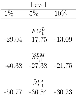
F GL1
-29.04 -17.75 -13.09
b
ST,LM1
-40.38 -27.38 -21.75
b
ST,Ld1
-50.77 -36.54 -30.23
F GL
1 is the wavelet test for no drift. SbT,LM1 and SbT,Ld1 are the wavelet tests for trend stationary
[image:23.612.241.370.275.435.2]alternatives without and with linear trends, respectively. Entries are based on one million Monte Carlo replications.
ρ 1% 5% 10% 1% 5% 10% 1% 5% 10%
b
ST,LM1 ERS MPP
γ=−0.80
1.00 0.009 0.068 0.119 0.014 0.047 0.097 0.011 0.045 0.099 0.99 0.982 0.997 0.998 0.156 0.401 0.587 0.144 0.402 0.610 0.98 1.000 1.000 1.000 0.451 0.702 0.827 0.443 0.704 0.840
γ=−0.50
1.00 0.006 0.045 0.103 0.011 0.051 0.102 0.011 0.049 0.108 0.99 0.668 0.871 0.937 0.148 0.396 0.569 0.141 0.393 0.592 0.98 0.984 1.000 1.000 0.487 0.746 0.846 0.479 0.748 0.863
γ= 0.00
1.00 0.006 0.046 0.087 0.013 0.052 0.099 0.011 0.052 0.106 0.99 0.153 0.486 0.687 0.163 0.423 0.596 0.156 0.416 0.611 0.98 0.683 0.954 0.991 0.488 0.741 0.846 0.495 0.743 0.855
γ= 0.50
1.00 0.006 0.038 0.085 0.015 0.055 0.112 0.013 0.053 0.118 0.99 0.069 0.316 0.543 0.168 0.422 0.605 0.162 0.417 0.619 0.98 0.374 0.845 0.953 0.475 0.715 0.844 0.473 0.721 0.856
γ= 0.80
[image:24.792.198.594.76.436.2]1.00 0.007 0.031 0.056 0.013 0.048 0.098 0.011 0.048 0.097 0.99 0.021 0.189 0.386 0.155 0.405 0.585 0.148 0.402 0.601 0.98 0.198 0.668 0.883 0.460 0.708 0.821 0.454 0.712 0.833
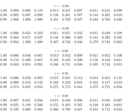
Table 2: Size and Power of the SbLM
T,1 - Demeaned Series with Serially Correlated Errors
The wavelet test statistic is calculated with a unit scale (J = 1) discrete wavelet transformation and with the Haar filter. The data generating process isyt=µ+yts, where yst =ρyts−1+ut,ut=γut−1+ǫt ǫt∼iidN(0,1), µ= 1 and y0 = 0. Under the null
ρ= 1 and under the alternativeρ <1. The asymptotic critical values of theSbLM
T,1 test are tabulated in Table 1. The bandwidth
is set to 20 with the Bartlett kernel in the calculation of the long-run variance of the wavelet test. The lag length of the ERS and MPP test regressions are determined by minimizing the modified AIC with the maximum lag length of 12. All simulations
ρ 1% 5% 10% 1% 5% 10% 1% 5% 10%
b
ST,Ld1 ERS MPP
γ=−0.80
1.00 0.002 0.054 0.124 0.014 0.047 0.095 0.012 0.047 0.098 0.99 1.000 1.000 1.000 0.141 0.379 0.565 0.123 0.374 0.582 0.98 1.000 1.000 1.000 0.410 0.679 0.810 0.406 0.684 0.828
γ=−0.50
1.00 0.002 0.056 0.121 0.012 0.053 0.101 0.011 0.049 0.103 0.99 0.854 0.963 0.984 0.154 0.415 0.586 0.151 0.411 0.602 0.98 0.996 0.999 0.999 0.467 0.714 0.825 0.471 0.721 0.836
γ= 0.00
1.00 0.001 0.054 0.112 0.010 0.052 0.103 0.008 0.053 0.103 0.99 0.152 0.496 0.697 0.152 0.412 0.571 0.141 0.406 0.587 0.98 0.580 0.895 0.971 0.474 0.717 0.824 0.473 0.719 0.835
γ= 0.50
1.00 0.001 0.048 0.112 0.007 0.049 0.092 0.007 0.048 0.094 0.99 0.014 0.226 0.480 0.173 0.427 0.580 0.162 0.420 0.593 0.98 0.090 0.583 0.810 0.470 0.716 0.828 0.467 0.719 0.839
γ= 0.80
[image:25.792.198.592.80.437.2]1.00 0.001 0.040 0.110 0.016 0.049 0.103 0.015 0.048 0.108 0.99 0.011 0.174 0.372 0.139 0.386 0.583 0.133 0.382 0.577 0.98 0.051 0.449 0.729 0.452 0.694 0.806 0.449 0.693 0.819
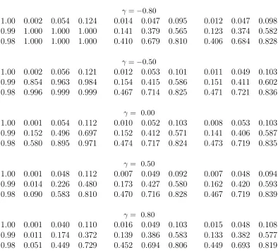
Table 3: Size and Power of the SbLd
T,1 - GLS Detrended Series with Serially Correlated Errors
The wavelet test statistic is calculated with a unit scale (J = 1) discrete wavelet transformation and with the Haar filter. The data generating process isyt=µ+αt+yts, where yts=ρyts−1+ut,ut=γut−1+ǫt ǫt∼iidN(0,1),µ= 1, α= 0.001 and y0 = 0.
Under the nullρ= 1 and under the alternative ρ <1. The asymptotic critical values of the SbLd
T,1 test are tabulated in Table 1.
The bandwidth is set to 50 with the Bartlett kernel in the calculation of the long-run variance of the wavelet test. The lag length of the ERS and MPP test regressions are determined by minimizing the modified AIC with the maximum lag length of
Figure 1: Wavelet Variance Decomposition of a White Noise Process
Energy (100%)
0.0 0.2 0.4 0.6 0.8 1.0
O
O
O
O
O
O
O
O Data
w1
w2
w3
w4
w5
w6
v6
(a)
Number of Coefficients
Cumulative Proportional Energy
1 5 10 50 100 500 1000
0.0
0.2
0.4
0.6
0.8
1.0
DWT Data
(b)
The energy decomposition of a white noise process through a six level discrete wavelet decomposition (DWT) with 1024
observations. (a)“Data” represents the total energy of the data which is normalized at one. wi, i= 1, . . . ,6 represents the percentage energy of the wavelet coefficients. v6 is the percentage energy of the scale coefficients. The energies of the wavelet
and scaling coefficients are equal to the sum of the energy of the data. The energy is the highest at the highest frequency
wavelet coefficient (w1) and declines gradually towards the lowest frequency wavelet coefficient (w6). The percentage energy of
the scaling coefficient (v6) is zero.(b)This figure compares the proportional energy of the data to the proportional energy of all coefficients. The number of coefficients needed is equal to the number of data points to account for the total energy of the
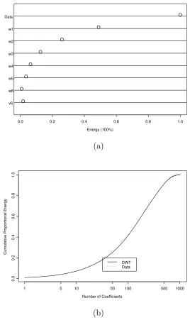
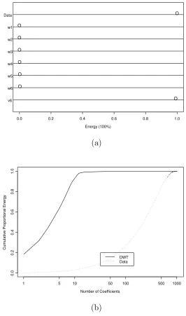
Figure 2: Wavelet Variance Decomposition of a Unit Root Process
Energy (100%)
0.0 0.2 0.4 0.6 0.8 1.0
O
O
O
O
O
O
O
O Data
w1
w2
w3
w4
w5
w6
v6
(a)
Number of Coefficients
Cumulative Proportional Energy
1 5 10 50 100 500 1000
0.0
0.2
0.4
0.6
0.8
1.0
DWT Data
(b)
The energy decomposition of a unit root process through a six level discrete wavelet decomposition (DWT) with 1024
observa-tions.(a)“Data” represents the total energy of the data which is normalized at one. wi, i= 1, . . . ,6 represents the percentage energy of wavelet coefficients. v6 is the percentage energy of the scaling coefficients. The energies of the wavelet and scaling
coefficients are equal to the sum of the energy of the data. The energy is the highest for the scaling coefficients and close to
zero for wavelet coefficients. The percentage energy of the scaling coefficients (v6) is close to the energy of the data.(b)This figure compares the proportional energy of the data to the proportional energy of all coefficients. The number of coefficients
References
Andrews, D. W. K. (1991). Heteroskedasticity and autocorrelation consistent covariance matrix estimation. Econometrica, 59, 817–858.
Berkes, I., Hormann, S., and Horvath, L. (2008). The functional central limit theorem for a family of garch observations with applications. Statistics & Probability Letters, 78, 2725–2730.
Bhargava, A. (1986). On the theory of testing for unit roots in observed time series. Review
of Economic Studies, 53, 369–384.
Cai, Y. and Shintani, M. (2006). On the alternative long-run variance ratio test for a unit root. Econometric Theory, 22, 347–372.
Chan, N. H. and Wei, C. Z. (1987). Asymptotic inference for nearly nonstationary AR(1) processes. Annals of Statistics, 15, 1050–1063.
Choi, I. and Phillips, P. C. B. (1993). Testing for a unit root by frequency domain regression.
Journal of Econometrics, 59, 263–286.
Coifman, R. R. and Donoho, D. L. (1995). Translation invariant denoising. Wavelets and
Statistics, ed. A. Antoniadis and G. Oppenheim, Vol. 103, New York, Springer-Verlag,
pages 125–150.
Daubechies, I. (1992). Ten Lectures on Wavelets, volume 61 of CBMS-NSF Regional
Con-ference Series in Applied Mathematics. SIAM, Philadelphia.
Davidson, R., Labys, W. C., and Lesourd, J.-B. (1998). Walvelet analysis of commodity price behavior. Computational Economics, 11, 103–128.
Dickey, D. A. and Fuller, W. A. (1979). Distributions of the estimators for autoregressive time series with a unit root. Journal of American Statistical Association, 74, 427–431.
Duchesne, P. (2006a). On testing for serial correlation with a wavelet-based spectral density estimator in multivariate time series. Econometric Theory,22, 633–676.
Duchesne, P. (2006b). Testing for multivariate autoregressive conditional heteroskedasticity using wavelets. Computational Statistics & Data Analysis, 51, 2142–2163.
Dufour, J. M. and King, M. (1991). Optimal invariant tests for the autocorrelation coefficient in linear regressions with stationary and nonstationary errors. Journal of Econometrics,
Elliott, G., Rothenberg, T. J., and Stock, J. H. (1996). Efficient tests for an autoregressive unit root. Econometrica, 64, 813–836.
Fan, Y. (2003). On the approximate decorrelation property of the discrete wavelet transform for fractionally differenced processes.IEEE Transactions on Information Theory,49, 516– 521.
Fan, Y. and Whitcher, B. (2003). A wavelet solution to the spurious regression of fractionally differenced processes. Applied Stochastic Models in Business and Industry,19, 171–183.
Gen¸cay, R., Sel¸cuk, F., and Whitcher, B. (2001). An Introduction to Wavelets and Other
Filtering Methods in Finance and Economics. Academic Press, San Diego.
Gen¸cay, R., Sel¸cuk, F., and Whitcher, B. (2003). Systematic risk and time scales.
Quanti-tative Finance, 3, 108–116.
Gen¸cay, R., Sel¸cuk, F., and Whitcher, B. (2005). Multiscale systematic risk. Journal of
International Money and Finance, 24, 55–70.
Granger, C. W. J. (1966). The typical spectral shape of an economic variable.Econometrica,
34, 150–161.
Hamilton, J. D. (1994). Time Series Analysis. Princeton University Press, Princeton, New Jersey.
Hong, Y. (2000). Wavelet-based estimation for heteroskedasticity and autocorrelation con-sistent variance-covariance matrices. Technical report, Department of Economics and Department of Statistical Science, Cornell University.
Hong, Y. and Kao, C. (2004). Wavelet-based testing for serial correlation of unknown form in panel models. Econometrica, 72, 1519–1563.
Hong, Y. and Lee, J. (2001). One-sided testing for ARCH effects using wavelets.Econometric
Theory,17, 1051–1081.
Lee, J. and Hong, Y. (2001). Testing for serial correlation of unknown form using wavelet methods. Econometric Theory, 17, 386–423.
MacKinnon, J. G. (2000). Computing numerical distribution functions in econometrics. High Performance Computing Systems and Applications, ed. A. Pollard, D. Mewhort, and D.
Mallat, S. (1989). A theory for multiresolution signal decomposition: The wavelet represen-tation. IEEE Transactions on Pattern Analysis and Machine Intelligence, 11, 674–693.
Mallat, S. (1998). A Wavelet Tour of Signal Processing. Academic Press, San Diego.
Nason, G. P. and Silverman, B. W. (1995). The stationary wavelet transform and some statistical applications.Wavelets and Statistics, Volume 103 of Lecture Notes in Statistics,
ed. A. Antoniadis and G. Oppenheim, Springer Verlag, New York, pages 281–300.
Nelson, C. R. and Plosser, C. I. (1982). Trends and random walks in macroeconomic time series: Some evidence and implications. Journal of Monetary Economics, 10, 139–162.
Newey, W. K. and West, K. D. (1987). A simple positive semidefinite heteroskedasticity and autocorrelation consistent covariance matrix. Econometrica, 55, 703–708.
Ng, S. and Perron, P. (2001). Lag length selection and the construction of unit root tests with good size and power. Econometrica, 69, 1519–1554.
Park, H. and Fuller, W. (1995). Alternative estimators and unit root tests for the autore-gressive process. Journal of Time Series Analysis, 16, 415–429.
Park, J. Y. and Phillips, P. C. B. (1988). Statistical inference in regressions with integrated processes: Part 1. Econometric Theory,4, 468–497.
Park, J. Y. and Phillips, P. C. B. (1989). Statistical inference in regressions with integrated processes: Part 2. Econometric Theory,5, 95–131.
Percival, D. B. (1995). On estimation of the wavelet variance. Biometrica, 82, 619–631.
Percival, D. B. and Mofjeld, H. O. (1997). Analysis of subtidal coastal sea level fluctuations using wavelets. Journal of the American Statistical Association, 92, 868–880.
Percival, D. B. and Walden, A. T. (2000). Wavelet Methods for Time Series Analysis. Cambridge Press, Cambridge.
Phillips, P. C. B. (1986). Understanding spurious regressions in econometrics. Journal of
Econometrics,33, 311–340.
Phillips, P. C. B. (1987a). Time series regression with a unit root. Econometrica, 55, 277–301.
Phillips, P. C. B. and Ouliaris, S. (1990). Asymptotic properties of residual based tests for cointegration. Econometrica, 58, 165–193.
Phillips, P. C. B. and Perron, P. (1988). Testing for a unit root in time series regression.
Biometrica,75, 335–346.
Phillips, P. C. B. and Solo, V. (1992). Asymptotics for linear processes. Annals of Statistics,
20, 971–1001.
Phillips, P. C. B. and Xiao, Z. (1998). A primer on unit root testing. Journal of Economic
Surveys, 12, 423–469.
Ramsey, J. B. (1999). The contribution of wavelets to the anlaysis of economic and financial data. Philosophical Transactions of the Royal Society of London A, 357, 2593–2606.
Ramsey, J. B. (2002). Wavelets in economics and finance: Past and future. Studies in
Nonlinear Dynamics & Econometrics, 3, 1–29.
Ramsey, J. B. and Zhang, Z. (1997). The analysis of foreign exchange data using waveform dictionaries. Journal of Empirical Finance, 4, 341–372.
Ramsey, J. B., Zaslavsky, G., and Usikov, D. (1995). An analysis of U. S. stock price behavior using wavelets. Fractals, 3, 377–389.
Sargan, J. D. and Bhargava, A. (1983). Testing residuals from least squares regression for being generated by the Gaussian random walk. Econometrica, 51, 153–174.
Schmidt, P. and Phillips, P. C. B. (1992). LM tests for a unit root in the presence of deterministic trends. Oxford Bulletin of Economics and Statistics, 54, 257–288.
Sims, C. A., Stock, J. H., and Watson, M. W. (1990). Inference in linear time series models with some unit roots. Econometrica, 58, 113–144.
Stock, J. H. (1995). Unit roots, structural breaks and trends. Handbook of Econometrics,
ed. R. F. Engle and D. McFadden, Amsterdam, North-Holland, pages 2739–2841.
Stock, J. H. (1999). A class of tests for integration and cointegration. Cointegration, Causal-ity, and Forecasting Festschrift in Honour of Clive W. J. Granger, ed. R. F. Engle and H.