Shooting Methods for Two-Point Boundary Value
Problems of Discrete Control Systems
G. Kishore Babu
Electriacl Engineering Dept. PSCMR Engineering College
Vijayawada, India 520002
M.S. Krishnarayalu,
Ph.DElectriacl & Electronics Engineering Dept. V R Siddhartha Engineering College
Vijayawada, India 520007
ABSTRACT
Two-point boundary value problems (TPBVP) are an important class of problems which appear frequently in optimal control. These may be well conditioned or ill conditioned. A well- conditioned TPBVP will have a system matrix with linearly independent columns due to closeness of its eigenvalues. On the other hand an ill conditioned TPBVP will have a system matrix with almost linearly dependent columns due to wide variation of its eigenvalues. In other words, a well- conditioned system is a one- time scale system whereas an ill conditioned system is a multi-time scale system. Ill conditioned systems are computationally stiff systems with widely separated eigenvalues. The stiffness increases with increase in time scales. The solution of TPBVP of discrete control systems is obtained by shooting method, that is, a number of initial value problems (IVP) will be shot to get the solution of TPBVP. The solution of a well-conditioned TPBVP is easier compared to an ill-well-conditioned
TPBVP. An ill-conditioned TPBVP requires
orthonormalization process to make the columns of the system matrix linearly independent. More the stiffness more the number of orthonormalization processes. Here the method of complimentary functions is used for well-conditioned systems and Conte's method for ill-conditioned systems. First we develop shooting methods for well-conditioned and ill-conditioned TPBVP of discrete control systems. Later the methods are supported with two illustrative examples one for each case.
Keywords
Discrete control, Time-scale systems, Optimal control, Stiff two-point boundary value problem, Shooting method, Orthonormalization
1. INTRODUCTION
For an nth order IVP n initial conditions are specified along with input. Hence IVP may be solved easily by recursive method starting from the initial data and input. However for TPBVP some boundary conditions are specified at initial time and the remaining at final time (or some other time). Hence they cannot be solved easily as IVP. A well- conditioned system is that one whose system matrix columns are linearly independent and whose inverse can be obtained easily. TPBVP may be solved using standard methods for well-conditioned systems. Some solution methods for TPBVP are Interpolation methods, Variational methods, Method of
Collocation, Picard’s method, Discrete methods,
Quasilinearization method and Shooting methods. However they may not work for ill-conditioned systems as it is. Also it is not possible to obtain a closed-form of solution practical TPBVP. Hence it is required to go for numerical methods. So much literature is available for TPBVP and multi-time scales of continuous-time systems [1-4].
Stiff two-point boundary value problems are frequently encountered in optimal control. Stiff systems are time-scale-systems or singularly perturbed time-scale-systems [5-14].The solution of two-point boundary value problems of stiff systems requires special methods such as shooting techniques. Shooting technique means finding the solution of BVP by shooting a number of IVP. Here an attempt is made to apply the same to discrete-time control systems.
2. STATEMENT OF PROBLEM
Consider an nth order linear shift invariant discrete system described by
x(k+1) = A x(k) + B u(k)
where
x(k) - nx1 state vector
u(k) - rx1 control vector
A – nxn system matrix
B – nxr input matrix
with boundary conditions
xj(k=0) = xj(0) j = 1,2, ..., m;
xj(k=N) = xj(N) j = m+1,m+2, ..., n. (1)
N is an integer indicating the final time.
This TPBVP is to be solved for different conditions of system matrix A. If all the eigenvalues of A are close to one another it is a well-conditioned problem from computational view. If the eigenvalues of A are widely scattered it results in time-scale behavior. The multi-time scale systems exhibit the phenomenon of chaos [4] and these are ill-conditioned systems from computational view. Next shooting methods are applied for TPBVP represented by (1) for well-conditioned and ill-conditioned cases.
2.1 Well-Conditioned TPBVP
17 Step 1: Homogeneous Solutions
For homogeneous solutions, Kronecker delta initial conditions are used as given below.
xh(1)[0]= 1 for m+1 else 0
xh (2)
[0] = 1 for m+2 else 0
…
xh (n-m)
[0]= 1 for n else 0
Shoot these IVPs and store the resulting data.
Step2: Particular solution
The initial condition for particular solution is given as
xf(0) = [x1(0) … xm(0)0…0]’
’ indicates transpose. Shoot and get the forced (particular) solution from xf(0) to xf(N)
Step 3: MIC
Here we compute the MIC.
MIC = 𝑥ℎ𝑏−1 *
𝑥𝑚 +1 𝑁 − 𝑥𝑓,𝑚 +1(𝑁)
𝑥𝑚 +2 𝑁 − 𝑥𝑓,𝑚 +2(𝑁)
… … 𝑥𝑛 𝑁 − 𝑥𝑓,𝑛(𝑁)
where
𝑥ℎ𝑏=
𝑥ℎ ,𝑚 +1 (1)
(𝑁) 𝑥ℎ,𝑚 +1(2) (𝑁) … 𝑥ℎ ,𝑚 +1(𝑛−𝑚 )(𝑁)
𝑥ℎ ,𝑚 +2(1) (𝑁) 𝑥ℎ,𝑚 +2(2) (𝑁) … 𝑥ℎ ,𝑚 +2(𝑛−𝑚 )(𝑁) …
𝑥ℎ ,𝑛(1)(𝑁)
… 𝑥ℎ ,𝑛(2)(𝑁) ……
… 𝑥ℎ ,𝑛(𝑛−𝑚 )(𝑁)
Step 4: Now solve the TPBVP as IVP using the given IC and MIC (that is shoot with IC and MIC).If MIC are accurate then the solution of x(k) satisfies all the given initial and final boundary conditions.
2.2 Ill Conditioned TPBVP
If the system matrix A is multi-time-scaled then the system becomes ill-conditioned and the columns of xhb will be almost linearly dependent. Hence xhb-1 and MIC cannot be computed
accurately. This problem can be overcome by
orthonormalizing xh at appropriate values of k.
Orthonormalizaion converts almost linearly dependent vectors into linearly independent vectors. Ill-conditioned TPBVP is solved using Conte’s algorithm employing complimentary
functions method along with Gram-Schmidt
orthonormalization process.
Gram-Schmidt orthonormalization process generates N orthonormal vectors𝑧(𝑖), 𝑖 = 1,2, … , 𝑁, from a set of N
linearly independent vectors 𝑥(𝑖), 𝑖 = 1,2, … 𝑁, by forming
linear combinations of the 𝑥(𝑖). The orthonormal set 𝑧(𝑖)has
the property
(𝑧(𝑗 ), 𝑧(𝑖)) = 1, j=i;
= 0, else
(𝑧(𝑗 ), 𝑧(𝑖)) is the inner product of the vectors 𝑧(𝑗 )𝑎𝑛𝑑𝑧(𝑖)and is
given by
(𝑧(𝑗 ), 𝑧(𝑖)) = 𝑧 𝑙 (𝑗 )
. 𝑧𝑙(𝑖)
𝑁
𝑙=1 . (2)
{η(𝑖)}
is the set of unnormalized orthogonal vectors which will be normalized to {𝑧(𝑖)}. The transformation from the x’s to the
z’s may be expressed in partitioned matrix form as Z=PX
𝑧(1)
⋮ 𝑧(𝑁)
=
𝑝11
⋮ ⋮
𝑝𝑁1 𝑝𝑁2 … 𝑝𝑁𝑁
𝑥
(1)
⋮ 𝑥(𝑁)
,
Z= Nx1 vector, whose elements are the vectors 𝑧(𝑁),
X=Nx1 vector, whose elements are the vectors 𝑥(𝑁),
P=NxN matrix of lower triangular form described by
𝑝𝑗𝑗 = 1/𝑤𝑗𝑗 j=i,
𝑝𝑗𝑖 = −
(𝑥(𝑗 ),𝑧(𝑠))
𝑤𝑗𝑗
𝑗 −1
𝑠=𝑖 𝑝𝑠𝑖, j>i,
𝑝𝑗𝑖= 0, j<i,
𝑤𝑗𝑗 = (η 𝑖 ,η(𝑖))1/2. (3)
Conte’s method
This algorithm uses the method of complementary functions. It is a two-phase method. In the first phase homogeneous and forced solutions are found out recursively as IVP using Kronecker delta initial conditions at appropriate values of k implementing Gram-Schmidt orthonormalization process. In the second phase the MIC are found out working backward. Next working forward, find the solution of the given BVP using IC and MIC as IVP. The algorithm is similar to that of continuous-time systems [1].
Notation: Let
H(q)(k) is an nx(n-m) matrix of solutions of the homogeneous equations xh(g,q)(k), g = 1,2,…n-m, which were last orthonormalized at kq, as shown below
H(q)(k) =
𝑥ℎ,1 (1,𝑞)
(𝑘) 𝑥ℎ,1(2,𝑞)(𝑘) … 𝑥ℎ,1(𝑛−𝑚 ,𝑞)(𝑘)
𝑥ℎ,2(1,𝑞)(𝑘) 𝑥ℎ,2(2,𝑞)(𝑘) … 𝑥ℎ,2(𝑛−𝑚 ,𝑞)(𝑘) …
𝑥ℎ,𝑛(1,𝑞)(𝑘) … 𝑥ℎ,𝑛(2,𝑞)(𝑘)
… …
… 𝑥ℎ,𝑛(𝑛−𝑚 ,𝑞)(𝑘)
(4)
P(q)’ = transpose of P(q), (n-m)x(n-m) matrix, which is the orthonormalization matrix of the homogeneous solutions
V(q)(k)= the particular solution last orthogonalized at kq.
Algorithm:
First phase
1. Set counter q=0 and time k=0. Using the Kronecker delta initial conditions compute homogeneous and particular solutions from k = 0 to k1 from steps 1&2 of well-conditioned TPBVP algorithm.
2. Set q=q+1. At kq, form the set of orthonormal vectors xh(g,q)(kq), g= 1,2,…n-m, from the set of(n-m) linearly independent vectors xh(g,q-1)(kq),g= 1,2,…n-m. In matrix form
H(q)(kq) = H(q-1)(kq)P(q)’
3. At kq, form the orthogonal complement of V(q-1)(kq) by subtracting out a linear combination of the orthonormal homogeneous vectors xh(g,q)(kq), g= 1,2,…n-m; as
V(q)(kq)=V(q-1)(kq)-H(q)(kq)ω(q)
where ω(q) = n-m x 1 vector with components
ω1(q),ω2(q),…,ωn-m(q), ωg
(q)
=(V(q-1)(kq),xh (g,q)
(kq)).
4. Compute recursively from kq to kq+1 the (n-m)
xh(g,q)(kq), g= 1,2,…n-m. Also compute particular solution from kq to kq+1starting with V(q)(kq).
5. If kq< N go to step 2.
6. At k = N execute steps 2 and 3. Here let Q=q+1 and kQ
= N
Second Phase
7. The general solution at N is given as the sum of the particular solution plus a linear combination of the homogeneous solutions.
x(kQ) = V(Q)(kQ) + H(Q)(kQ) βQ corresponding to n-m terminal boundary conditions.
Solving βQ=H(Q)(kQ)-1[x(kQ) - V(Q)(kQ)].
βQ = (n-m) x 1 vector of constants with components
β1(Q),β2(Q),…,βn-m(Q).
8. The MIC corresponding to n-m terminal boundary
conditions is constructed by working backward from N as
β(q-1)
= P(q)’[β(q)-ω(q)], q = Q, Q-1, …, 1.
where P(q), and ω(q) have been computed in first phase.
β(0)
is the MIC.
9. Perform final shoot with given IC and MIC to get the required solution of TPBVP.
3. ILLUSTRATIVE EXAMPLES
Two examples are provided in support of the shooting methods for TPBVP; one for well-conditioned discrete control system which does not require orthonormolization and other for ill-conditioned discrete control system which requires orthonormolization. The results are given in tabular form.
3.1 Example I
Consider the third order single area power system model used for LFC sampled with 0.2s [12]. The resulting system is given by
𝑥01 𝑘 + 1
𝑥02 𝑘 + 1
𝑥1 𝑘 + 1
=
0.772 0.037 −0.017
0.085 0.720 0.0406
−0.244 0.145 0.0306
𝑥01 𝑘
𝑥02 𝑘
𝑥1 𝑘
+
−0.144 0.074 0.705
u(k) (5)
Here 𝑥0=
𝑥01
𝑥02 and u(k) is unit step function. The Eigen
spectrum of this system
(0.8078, 0.6992, 0.0156)
clearly indicates two-time-scale nature with two slow modes represented by x0and one fast mode represented by x1.
The boundary conditions are given as
x01(10) =1; x02(10) = 1; x1(0) = 10. (6)
Here n = 3 and m = 1. By applying the shooting method of well-conditioned systems developed in Section 2.1, the solution obtained from MATLAB programming is given below. Please note that all the boundary conditions are satisfied.
Step 1: Homogeneous solutions xh
(1)
[0] = [1;0;0] using MATLAB notation
xh(2)[0] = [0;1;0]
The resulting final values at k =10, after shooting, are
xh(1)[10] = [0.0932; 0.0596;-0.0191]
xh(2)[10] = [0.0278;0.0524;0.0021]
Step2: Particular solution
The initial condition for particular solution is given as
xf(0) = [0;0;10]
The resulting final values at k =10, after shooting, are
xf(10) = [-0.6183; 0.2430;0.9185]
Step 3: MIC
The resulting 𝑥ℎ𝑏 and MIC are
𝑥ℎ𝑏 =0.0932 0.02780.0596 0.0524
MIC = [19.7476; -7.9997]
Step 4: Shoot with initial conditions and MIC
x01(0) =19.7476; x02(0) = -7.9997; x1(0) = 10.
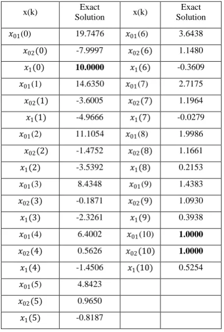
[image:3.595.309.538.398.737.2]The resulting solution is shown in Table1. As seen from this table all boundary conditions x01(10) =1, x02(10) = 1, x1(0) = 10 (indicated in boldface) are satisfied. Hence this is the solution of given TPBVP. The same results are displayed in Fig. 1 giving picturesque view.
Table 1 – TPBVP solution for well-conditioned system
x(k) Exact
Solution x(k)
Exact Solution
𝑥01(0) 19.7476 𝑥01(6) 3.6438
𝑥02(0) -7.9997 𝑥02(6) 1.1480
𝑥1(0) 10.0000 𝑥1(6) -0.3609
𝑥01(1) 14.6350 𝑥01(7) 2.7175
𝑥02(1) -3.6005 𝑥02(7) 1.1964
𝑥1(1) -4.9666 𝑥1(7) -0.0279
𝑥01(2) 11.1054 𝑥01(8) 1.9986
𝑥02(2) -1.4752 𝑥02(8) 1.1661
𝑥1(2) -3.5392 𝑥1(8) 0.2153
𝑥01(3) 8.4348 𝑥01(9) 1.4383
𝑥02(3) -0.1871 𝑥02(9) 1.0930
𝑥1(3) -2.3261 𝑥1(9) 0.3938
𝑥01(4) 6.4002 𝑥01(10) 1.0000
𝑥02(4) 0.5626 𝑥02(10) 1.0000
𝑥1(4) -1.4506 𝑥1(10) 0.5254
𝑥01(5) 4.8423
𝑥02(5) 0.9650
19
Fig. 1 Solution of Illustrative Example I
3.2 Example II
Consider the TPBVP resulting from two-parameter optimal control [14]
𝑥01 𝑘 + 1
𝑥02 𝑘 + 1
𝑥11 𝑘 + 1
𝑥12(𝑘 + 1)
𝑥2(𝑘 + 1)
𝑝01 𝑘
𝑝02 𝑘
𝑝11 𝑘
𝑝12(𝑘)
𝑝2(𝑘)
=
0.9147 0.0253 0.0125 0.0075 0.0051
−0.0602 0.8893 −0.0003 0.4560 0.0295
−0.0195 0.7016 0.2465 0.0209 0.0192
−1.4300 −0.0219 −0.0138 0.2399 −0.0063
−1.1124 −0.0125 −0.0089 0.3388 0.0259
−0.0000 −0.0005 −0.00002 −0.0029 −0.0002
−0.0005 −0.0037 −0.00024 −0.0184 −0.0014
−0.0001 −0.0145 −0.0111
−0.0012 −0.0924 −0.0711
−0.00006 −0.0059 −0.0004 −0.00594
−0.0045 −0.4503 −0.3465
−0.0346 −0.0266 0.2500 0.0000 0.0000 0.0000 0.0000
0.0000 0.2500 0.0000 0.0000 0.0000 0.0000
0.0000 0.0000
0.0000 0.0000 0.0000
0.1500 0.0000 0.0000 0.0000
0.0000 0.1500 0.0000
0.0000 0.0200
0.9147 −0.0602 −0.0039 −0.2860 −0.0222
0.0253 0.8893 0.1403 −0.0043 −0.0002
0.0625 0.0375 0.2550
−0.0015 0.2280 1.47500
0.2465 −0.0138 −0.0009 0.0209
0.1920
0.2399 0.0338 −0.0630 0.0259
𝑥01 𝑘
𝑥02 𝑘
𝑥11 𝑘
𝑥12(𝑘)
𝑥2(𝑘)
𝑝01 𝑘 + 1
𝑝02 𝑘 + 1
𝑝11 𝑘 + 1
𝑝12(𝑘 + 1)
𝑝2(𝑘 + 1)
with boundary conditions
x01(0) = 2; x02(0) = -1; x10(0) = 1; x12(0) = 5; x2(0) = -4 and p01(6) = 0; p02(6) = 0; p11(6) = 0; p12(6) = 0; p2(6) = 0
(7)
Eigen values of this TPBVP are
{33.84855; 4.08196 ± 0.40125i; 1.13125 ± 0.10143i; 0.87692 ± 0.07862i; 0.242635 ± 0.02385i; 0.029543}
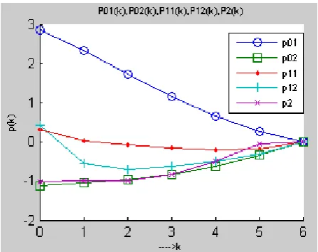
[image:4.595.60.276.71.215.2]This clearly indicates stable and unstable slow, fast and faster modes. This system is a true multi-time-scale system with chaotic behavior exhibiting butterfly phenomenon. The optimal solution is obtained by Conte’s method as mentioned in Section 2.2 Ill-conditioned TPBVP. The result is shown below in Table 2 for this numerical method. Also it is displayed pictorially in Figures 2 and 3 for quick view. Fig. 2 shows the solution of states x(k) whereas Fig. 3 displays the solution of co-states p(k).
Table 2 – TPBVP solution for ill-conditioned system
x(k)&p(k) Optimal
Solution x(k)&p(k)
Optimal Solution
x01(0) 2.00000 p01(3) 1.16381
x02(0) -1.00000 p02(3) -0.84362
x11(0) 1.00000 p11(3) -0.14593
x12(0) 5.00000 p12(3) -0.63653
x2(0) -4.00000 p2(3) -0.82417
p01(0) 2.86755 x01(4) 1.24857
p02(0) -1.11978 x02(4) -1.24329
p11(0) 0.31332 x11(4) -1.14097
p12(0) 0.43092 x12(4) -2.32278
p2(0) -1.02475 x2(4) -2.27450
x01(1) 1.83594 p01(4) 0.66903
x02(1) -0.88573 p02(4) -0.62869
x11(1) -0.46181 p11(4) -0.19641
x12(1) -1.27960 p12(4) -0.49655
x2(1) -0.36337 p2(4) -0.49148
p01(1) 2.32156 x01(5) 1.06844
p02(1) -1.05230 x02(5) -1.34642
p11(1) 0.03291 x11(5) -1.26783
p12(1) -0.55425 x12(5) -2.11286
p2(1) -1.00144 x2(5) -2.07634
x01(2) 1.64240 p01(5) 0.26711
x02(2) -0.94998 p02(5) -0.33660
x11(2) -0.79927 p11(5) -0.19017
x12(2) -2.48652 p12(5) -0.31693
x2(2) -2.14862 p2(5) -0.04152
p01(2) 1.72688 x01(6) 0.90095
p02(2) -0.97576 x02(6) -1.41891
p11(2) -0.07234 x11(6) -1.36202
p12(2) -0.70535 x12(6) -1.97468
p2(2) -0.99976 x2(6) -1.93003
x01(3) 1.44111 p01(6) 0.00000
x02(3) -1.10474 p02(6) 0.00000
x11(3) -0.98380 p11(6) 0.00000
x12(3) -2.52265 p12(6) 0.00000
x2(3) -2.41595 p2(6) 0.00000
[image:4.595.49.270.687.769.2]Fig. 3 Solution of Co-States p(k) of Illustrative Example II
4. CONCLUSIONS
TPBVP occur in many engineering problems like optimal control. TPBVP solution is not easy as the response has to satisfy both the initial and terminal boundary conditions. Their solution is easy for well-conditioned systems compared to ill-conditioned systems. These methods are available for continuous systems. Here they are presented for discrete control systems with two illustrative examples one for well- conditioned and one for ill-conditioned TPBVP. Method of complimentary functions is used for well conditioned TPBVP. Ill-conditioned TPBVP is solved using Conte’s method employing complimentary functions method along with Gram-Schmidt orthonormalization process. Start with orthonormalizing at k=N. If it is not yielding accurate MIC and TPBVP solution, then orthonomalize at k=N/2 and N for even N. If this also not yielding the required TPBVP solution then orthonormalize at k=N/4, 2N/4, … and N for even N. And so on. Similar selection may be employed for odd N. The numbers of orthonormaliztions depend upon the degree of ill-condition of A matrix. If the system is more ill-conditioned more the number of orthonormaliztions required.
5.
ACKNOWLEDGMENTS
We greatly acknowledge Siddhartha Academy of General and Technical Education, Vijayawada for providing the facilities to carry out this research.
6.
REFERENCES
[1] Roberts S.M. and Shipman J.S. (1972) Two-point
Boundary Value Problems: Shooting Methods. Elsevier, New York.
[2] SUNG N. HA, ”A Nonlinear Shooting Method for
Two-Point Boundary Value Problems” Computers and Mathematics with Applications 42 (2001) 1411-1420.
[3] Dinkar Sharma, Ram Jiwari, SheoKumar, ”Numerical
Solution of Two Point Boundary Value Problems Using Galerkin-Finite Element Method” ISSN 1749-3889 (print), 1749-3897 (online) International Journal of Nonlinear Science Vol.13(2012) No.2,pp.204-210.
[4] Koichi F. and Kunihiko K. (2003). Bifurcation cascade as chaotic itinerancy with multiple time scales. Chaos: An Interdisciplinary Journal of Nonlinear Science, 13, 1041-1056.
[5] Naidu D. S. (2002), Singular Perturbations and Time Scales in Control Theory and Applications: An Overview. Dynamics of Continuous, Discrete & Impulsive Systems, 9, 2, 233-278.
[6] Naidu, D.S and Rao, A.K. (1985), Singular perturbation analysis of discrete control systems. Volume 1154 of Lecture Notes in Mathematics, A.Dold and B. Eckmann, eds, Springer-Verlag.
[7] Naidu, D.S and D.B Price (1988), Singular perturbations and time scales in the design of digital flight control systems. NASA Technical paper 2844.
[8] Krishnarayalu M. S. (1989), Singular perturbation
method applied to the open-loop discrete optimal control problem with two small parameters. Int. J. Systems Science, 20, 5, 793-809.
[9] Krishnarayalu M. S. (1994), Singular perturbation
analysis of a class of initial and boundary value problems in multiparameter digital control systems. Control- Theory and Advanced Technology, 10, 3, 465-477.
[10]Krishnarayalu M. S. (1999), Singular perturbation methods for one-point, two-point and multi-point boundary value problems in multiparameter digital control systems. Journal of Electrical and Electronics Engineering, Australia, 19, 3, 97-110.
[11]Krishnarayalu M. S. (2008), Singular perturbation method applied to the discrete Euler-Lagrange free-endpoint optimal control problem. Automatic Control (theory and applications) AMSE journal, 63, 3, 16-29.
[12]Kishore Babu G. and Krishnarayalu M. S.(2014) Some Applications of Discrete One Parameter Singular Perturbation Method. JCET Vol. 4 Iss.1, PP. 76-81.
[13]Calovic, M. (1971), Dynamic State Space Models of Electric Power Systems(Urbana: University of Illinois Press).
[14]Kishore Babu G. and Krishnarayalu M. S.(2014)